Device Anomaly Detection Algorithm Based on Enhanced Long Short-Term Memory Network

LUO Xin(罗 辛), CHEN Jing(陈 静), YUAN Dexin(袁德鑫), YANG Tao(杨 涛)

1 School of Computer Science and Technology, Donghua University, Shanghai 201620, China 2 School of Continuing Education &School of Network Education, Donghua University, Shanghai 200051, China

Abstract：The problems in equipment fault detection include data dimension explosion, computational complexity, low detection accuracy, etc. To solve these problems, a device anomaly detection algorithm based on enhanced long short-term memory (LSTM) is proposed. The algorithm first reduces the dimensionality of the device sensor data by principal component analysis (PCA), extracts the strongly correlated variable data among the multidimensional sensor data with the lowest possible information loss, and then uses the enhanced stacked LSTM to predict the extracted temporal data, thus improving the accuracy of anomaly detection. To improve the efficiency of the anomaly detection, a genetic algorithm (GA) is used to adjust the magnitude of the enhancements made by the LSTM model. The validation of the actual data from the pumps shows that the algorithm has significantly improved the recall rate and the detection speed of device anomaly detection, with the recall rate of 97.07%, which indicates that the algorithm is effective and efficient for device anomaly detection in the actual production environment.

Key words：anomaly detection; production equipment; genetic algorithm (GA); long short-term memory (LSTM); principal component analysis (PCA)

0 Introduction

With the rapid development of the manufacturing industry, the stable and efficient operation of the equipment for production is important to improve production efficiency and save production costs, and it is necessary to detect abnormalities in the operation status of the equipment. A number of scholars and industry personnel in China and abroad are currently engaged in research on device anomaly detection[1], proposing methods that combine traditional statistical theory with machine learning, as well as deep learning detection methods[2].

Anomaly detection can be defined as finding abnormal data points in the data that deviate from normal behaviors, and it depends on the application domain. These “deviations” can also be called anomalies, outliers, or singularities. The traditional method of statistical theory usually takes the statistical distribution in statistics as the criterion of abnormal judgment. By using these methods, the mean, variance, median and plural of statistical data are calculated. After its error is verified to obey the probability distribution model such as Gaussian distribution, it is determined whether the data is abnormal according to the central limit theorem and significant difference. This analysis method is simple and practical, and it maintains good monitoring efficiency for equipment in normal conditions. However, it cannot consider variable environmental and operating conditions, and cannot adapt to different working conditions of different equipment. Machine learning-based methods perform data analysis by means of temporal predictive analysis and clustering analysis. The temporal predictive methods are modeled based on certain regularity or periodicity presented by the data[3-4], but their anomaly detection models often lack generalization ability for cases without regularity or periodicity. The clustering methods require a large amount of normal data as well as anomalous data[5], but in the actual production environment, the collection of data samples is too difficult due to the low probability events of anomalous data.

In recent years, with the rapid development of data processing capabilities, big data and artificial intelligence technologies have been rapidly applied in practice, and the field of deep learning methods for anomaly detection has received extensive attention from more and more researchers and scholars[6-7]. Deep learning networks typically consist of multiple hidden layers, and they can learn to capture nonlinear relationship in data by adjusting their own parameters, theoretically allowing them to approximate any complex function.The multilayer structure can extract more advanced features of the data to achieve the extraction and expression of the hidden information of the data itself and get the description of the results expected.

Due to the characteristics of unstable, nonlinear, and dynamically changing time-series data, deep learning-based methods still face problems such as difficulty in determining the optimal network parameters, noise interference in the data, and high computational complexity. The anomaly time of the observed data is not regular and their anomalies do not occur at the same moment, which makes it difficult to define the anomalous parameters based on the data. The noise generated in the input data is also difficult to use for noise reduction or denoising like image data because the noise not generated by the anomaly can contribute significantly to the calculation of the anomaly level instead. In addition, as the length of the time-series data increases, the time required for the computation and the complexity of the data also increases, which can lead to a subsequent increase in the computational complexity and the difficulty of the neural network. The long short-term memory (LSTM) network algorithm solves the gradient disappearance and gradient explosion problems relative to traditional neural networks and can handle long-term dependency. It specifically refers to the challenge of capturing and modeling dependency that exists among the elements far apart in a sequence data. The LSTM network algorithm overcomes this challenge by utilizing the memory mechanism of cell states, allowing the network to learn more complex sequence information[8-9].

To address the above problems, an enhanced LSTM network algorithm is proposed to break through the limitation of shallow deep learning network models in feature characterization at the network layer, making it challenging to distinguish the fault samples in the noisy environment due to the high dimensionality of data and mixed with a large amount of environmental noise in the actual industrial environment. Firstly, the principal component analysis (PCA) algorithm is applied to reduce the dimensionality of sensor data to extract the correlation between data with less noise and redundancy and reduce the computational complexity of the neural network algorithm[10-11], and then the memory mechanism of the enhanced LSTM model is used to predict the data of future periods or current periods by the data of previous periods to better discover the potential patterns of time series datasets. The genetic algorithm (GA) is used during the period to find the solution with the highest fitness for the augmented parameters in the LSTM network to optimize the training results. Finally, the algorithm is validated by pump data to be effective in the process of anomaly detection in real production equipment.

1 Real Device Sensor Timing Data Correlation Analysis

To analyze the correlation of sensor timing data of real equipment, a dataset from the Kaggle competition website is used to conduct experiments on a water pumping system of small town waterworks which fail seven times a year. These failures cause inconvenience to many households. The dataset includes measurement data from 51 sensors, including sensing of 5 types: pressure, lift, shaft power, flow rate and speed (Fig.1). The distribution of the data is shown in Fig.2. The total amount of data is 220 320, including 7 fault data (broken), 14 477 fault recovery status data (recovering), and 205 836 normal status data (normal).

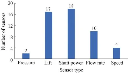
Fig.1 Distribution of sensor types

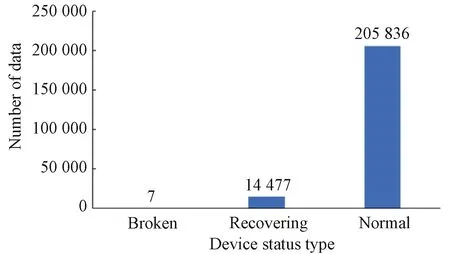
Fig.2 Distribution of data

To analyze the abnormal status of sensor timing data, the sensor measurement data in 5 months are intercepted for visual analysis(Fig.3). The red marked point in Fig.3 means the fault occurrence. From Fig.3, it can be seen that the data at the moment of failure of the sensors change abruptly and deviate from the normal range of the original values. Therefore, the abnormal condition of the equipment can be predicted by the measurement data of different sensors.

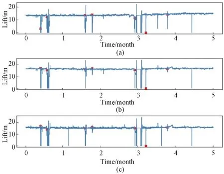
Fig.3 Partial head dataset fault point status: (a)sensor_06; (b)sensor_07; (c)sensor_08

Since the equipment components work in conjunction, for example, the indicator of the maximum height that the pump can lift, the headHis usually related to the flow rate, pressure and other factors. It is clear that the data from different types of sensors must be correlated to some extent.

The formula for calculating the headHis

(1)

wherep1andp2represent the pressure of the liquid at the pump inlet and the pump outlet, respectively;c1andc2represent the flow rate of the fluid at the pump inlet and the pump outlet, respectively ;z1andz2represent the height of the inlet and the outlet, respectively;ρrepresents the density of the liquid;grepresents the acceleration of gravity.

For the dataset, the relationship mapping drawn by traversing each sensor data is shown in Fig.4, indicating the distribution of each sensor correlation relationship, such as pressure (sensor_00) and shaft power (sensor_04). The darker the color of the vertical and the horizontal intersection grid areas beyond the diagonal, the larger the corresponding relationship value, which indicates a stronger relationship between the sensors. According to the color shades presented by their intersection points against the color labeled values on the right, it can be judged that the relationship values of sensors with strong correlation are above 0.850, which shows that there is a fairly high linkage between these sensor data.

According to the analysis results, it can be seen that the equipment sensor measurement dataset represented by the pump has a complex form and a large amount of data, which increases the complexity and difficulty of the calculation. If the strong correlation data between the sensor data is extracted and the weak correlation data in the data is reduced, the purpose of dimensionality reduction can be achieved and the noise and redundancy can be reduced, thus reducing the complexity of the neural network algorithm calculation and improving the learning efficiency.

2 Enhanced LSTM-Based Device Anomaly Detection Algorithm

In real industrial environments where the equipment sensor timing data is highly dimensional and mixed with a large amount of environmental noise, shallow deep-learning network models are limited by the feature characterization capability of the network layer, and it is not easy to distinguish the fault sample problems in noisy environments. To address this problem, an enhanced LSTM network classification algorithm, the PCA-GA-LSTM algorithm, is proposed in this paper to better utilize contextual information for prediction. The framework of the PCA-GA-LSTM algorithm (Fig.5) includes a data processing module, a parameter optimization module, a data training module and a data prediction module. Specifically, the data processing module uses the PCA algorithm to reduce the dimensionality of the normalized data and then divides the dataset. The parameter optimization module enhances the LSTM network by GA. The data training module uses the enhanced LSTM network for training. The data prediction module uses the trained network to make predictions on real datasets.

2.1 PCA-based data processing module

In extracting the production equipment sensor feature parameters, the rich number and the type of sensors reflect the state of the equipment from different aspects, but there are very weakly correlated redundant information and noise between these parameters. The data processing module, through PCA, maps the originaln-dimensional features tok-dimensionnal features (n>k), replaces the original variables by linear combinations between the original variables, realizes high dimensional data for dimensionality reduction, retains more information of strongly correlated data[12], and minimizes the weakly correlated information to reduce the complexity of computation.

The dataset used in this paper hasmsamples {x1,x2,…,xm} and each sample hasnfeaturesxi=[xi,1,xi,2,…,xi,n]T.The original data are formed into ann×mmatrixXby columns. The specific dimensionality reduction steps are shown in Fig.6.

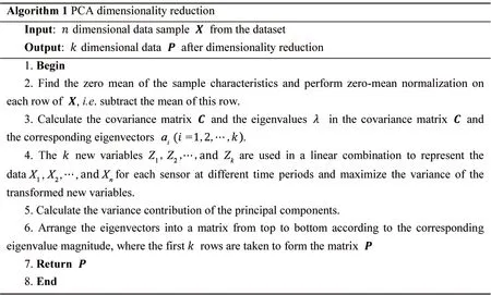
Fig.6 PCA dimensionality reduction steps

The input of the GA in this paper is then-dimensional data of the dataset, and the output is thek-dimensional data after dimensionality reduction. The specific calculation process is as follows.

1) Locate the zero mean of the sample attributes. Apply zero-mean normalization to individual rows of matrixXby subtracting the corresponding row mean from each element.

2) Calculate the covariance matrixCusing the eigenvaluesλias defined in equationC, along with their corresponding eigenvectors represented byαi(i=1,2,…,k).

3) Blend theknewly derived variablesZ1,Z2, ..., andZkin a linear fashion to effectively capture the data emanating from each sensorX1,X2, …, andXnacross various temporal segments. Strive to optimize and compute the variance inherent in these transformed variables using the provided formula.

4) Compute the proportion of the variance attributed to the principal component.

It is proved that the larger the contribution, the higher the degree of importance. The variance of thekth principal component is equal to thekth eigenvalueλkof the covariance matrix, and the variance contributionVkis calculated as

(2)

whereVkis the variance contribution of thekth principal component;λiis theith eigenvalue of the covariance matrix.

5) Arrange the eigenvectors into a matrix according to the corresponding eigenvalue size from top to bottom. The firstkrows are taken to form the matrixP.Zis the data after dimensionality reduction tokdimensions,i.e.Z=PX.

In order to verify the effectiveness of dimensionality reduction, the visualization analysis of dimensionality reduction of the experimental dataset is carried out in this paper based on the above principles. Figure 7(a) shows the dimensionality reduction of the dataset to two dimensions, with the horizontal axis representing variablex1and the vertical axis representing variablex2. Figure 7(b) shows the visualization image of the dimensionality reduction of the dataset to three dimensions, with the three axes beingx1,x2andx3. In Fig.7, the red part indicates the data at normal moments and the blue part indicates the data at abnormal moments. It can be seen from the visualization image analysis that the variables after the dimensionality reduction retain strong correlations. All moment dataxi=[xi,1,xi,2,…,xi,n]Tcan be reduced from 51 dimensions to two-dimensional (xi=[xi,1,xi,2]T) or three-dimensional (xi=[xi,1,xi,2,xi,3]T) as shown in Fig.6, which can significantly improve the efficiency of the calculation.

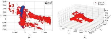
Fig.7 Schematic diagram of data after dimensionality reduction: (a) visualization of dataset downscaled to 2 dimensions; (b) visualization of dataset downscaled to 3 dimensions

However, a low dimensionality of the data can cause a large amount of information loss and affect the prediction accuracy, and it is also an issue to be considered to improve the efficiency of calculation and ensure the validity of the data. In this paper, the algorithm selects the dimensions of dimensionality reduction by the cumulative contribution rate, which represents the degree of reflection of the original data. The higher the value, the more it can reflect the information contained in the original data. The formula for calculating the cumulative contribution rate of each principal component is

(3)

whereTVis the cumulative contribution rate;Vkis the variance contribution of thekth principal component;λjis thejth eigenvalue of the covariance matrix.

In general, a cumulative contribution rate of 85%-95% can reflect the information of the vast majority of the data[12]and effectively reduce the dimensionality of the original data, so variables with a contribution rate of 90% or more are used as inputs to the model in this paper.

2.2 Enhanced LSTM data training module

2.2.1EnhancedstackedLSTMnetworkstructure

Deep recurrent neural networks provide empirical advantages beyond shallow networks[13], and in this paper, we propose an enhanced stacked LSTM network model that is compatible with the nonlinearity and complexity of time series data. On the one hand, we establish an enhanced stacked LSTM network to discriminate faulty samples in noisy environments by deepening the number of LSTM layers. On the other hand, we increase the number of fully connected layers and adjust the number of neurons to enhance the fit of the network to the data.

Figure 8 shows the enhanced stacked LSTM network model proposed in this paper, where LSTM blocks are connected to the deep recurrent networks one by one to form the stacked LSTM layers and combine the advantages of individual LSTM layers. Each layer contains multiple cells to process the timing data. In the stacked LSTM layer, the sensor dataXtat timetis introduced into a second LSTM block with a previously hidden stateht-1. The hidden statehtat timetis computed as described in the previous section and then moved to the next time step, also rising to the second LSTM layer. Such a structure allows the states of each layer to operate at different time scales. It also allows for performing layering in time-based processes and storing data sequence structures more naturally, and the enhanced multilayer network model effect is evident when there are long-term dependent production equipment data or temporal datasets from multivariate sensors[14-15].

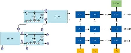
Fig.8 Enhanced stacked LSTM network model

Each LSTM cell is computed as follows.

Firstly, the reduced-dimensional sensor sequence,i.e., the column vectorXtcontainingkelements, is passed into the LSTM structure at each moment. The forgetting gate decides which information in the sensor sequence data should be discarded or retained at that moment. The output value obtained is between 0 and 1, and the closer the value obtained is to 1, the more it indicates that it should be retained.

ft=σ(WfXt+Ufht-1+bf),

(4)

whereftis the value of the forgetting gate;WfandUfare the weight matrices of the forgetting gate;ht-1denotes the hidden state at timet-1;bfdenotes the bias vector of the forgetting gate.WfandUfare used respectively to control the degree of the forgetting for the information from the input state at timetand the hidden state at timet-1.

The input gate is used to update the cell state. The information ofht-1is passed to the sigmoid function after connecting it with the sensor sequencextinput at the current moment to adjust the degree of retention of the hidden information, as shown in Eq. (5).

it=σ(WiXt+Uiht-1+bi),

(5)

whereitis the value of the input gate;WiandUiare the weight matrices of the input gate;bidenotes the bias vector of the input gate.WiandUiare used respectively to control the degree of retention for the information from the input state at timetand the hidden state at timet-1.

C′t=tanh(WcXt+Ucht-1),

(6)

Ct=ftCt-1+itC′t,

(7)

whereCtandC′tare the update content and alternative update content, respectively.WcandUcare used respectively to represent the level of attention to the input state at timetand the hidden state at timet-1, in order to subsequently update content based on the forgetting gate and the input gate.

Finally, after getting the updated value of the cell stateCt, the statehtat the current timetcan be generated based on the new cell state and is used to calculate the output of the current model or to participate in the input of the next layerht+1. The output gate of the hidden layer is expressed as Eq.(8), and then the output value of the LSTM network at the momenttcan be obtained by Eq. (9).

Ot=σ(woXt+Uo+ht-1+bo),

(8)

ht=Ottanh(Ct),

(9)

whereOtdenotes the output value,σdenotes the sigmoid function,Uois the weight matrix of the output stateOt; storing all useful information at timetand before;bodenotes the bias vector.

Since the output results of traditional LSTM networks are mapped to one layer of fully connected layers or the number of neurons is too small, it will lead to the limitation of its final fitting ability, and when complex functions need to be fitted, it often shows insufficient fitting ability, slow convergence in the training phase of the model, severe fluctuation, and large prediction error. Therefore, we add a multilayer fully connected layer network to the output layer of the stacked LSTM network model and adjust the number of neurons to enhance the fitting ability of the network, thus forming an enhanced stacked LSTM network model and reducing the volatility and error of the prediction results.

2.2.2ParameterdebuggingmethodbasedonenhancedstackedLSTMnetworkmodel

2.2.2.1 Optimization algorithm

A good default implementation of gradient descent is the Adam algorithm. This is because it combines the best properties of AdaGrad and RMSProp methods and automatically uses a custom learning rate for each parameter (weight) in the model.

2.2.2.2 Activation functions

The activation function is usually fixed by the frame and the scale of the input or output layer. For example, an LSTM uses a sigmoid activation function for the input, so the input is usually scaled from 0 to 1.

2.2.2.3 Regularization

LSTM can converge quickly or even overfit on some sequence prediction problems. To solve this problem, regularization methods can be used. The dropout randomly skips neurons during training, forcing other neurons in the layer to select the remainder.

2.2.3DatatrainingbasedonenhancedLSTMnetwork

2.2.3.1 Data input

After the device sensor data are dimensioned down by PCA in the data processing layer, the result of the dimensionality reduction is ak-dimensional temporal dataXtcomposed of multiple sensors linearly, and the divided sensor dataXtof different moments are passed into the LSTM network, and the training process based on the LSTM network is shown in Fig.9. Assuming that the incoming time series is the entire sensor dataset, there aretsequences, each consisting of a column vector ofkelements, and because there aretsequences, the LSTM requiresttime steps (i.e.,ttimes of self-loops) to complete the sequence.

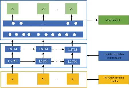
Fig.9 Model training based on enhanced LSTM network

2.2.3.2 LSTM layer training

The incoming sensor dataXt-1is processed by the weightsWand biasbin the LSTM gate structure to obtain the hidden statehtpassed to the next step, which connects the hidden layer output of the previous step with the inputXtof this layer and obtainsht+1by calculation. Thenht+1is passed to the next step and rises to the second LSTM layer. After multilayer multi-step processing, the output value of the LSTM network layer is finally obtained.

2.2.3.3 Abnormal output

After learning the relationship between the sensor sequence data and the equipment system fault through the LSTM layer, the learned information is passed to the multilayer fully connected layer behind for processing. It combines all the features learned by the previous LSTM layer and passes them to the output layer through weighted summation, and if the state of the equipment represented by the set of sensor data is judged to be normal, the output result is 0.

2.3 GA-based parameter optimization module

The number of fully connected layers, the number of stacked LSTM layers, and the number of neurons in the enhanced LSTM network model are all important factors affecting the training effect of the network, and the optimal parameters need to be chosen to achieve the best training effect. GA is a global optimization algorithm that overcomes the drawback of general numerical solution methods such as iterative operations, which tend to fall into the trap of local minima and become “dead loops” that prevent further progress[16-17]. GA can be used to obtain optimal solutions for the parameters of the augmented LSTM network to improve the accuracy of anomaly detection in neural networks[18-20]. In this paper, GA is used to select the number of network layers, the number of fully connected layers, and the number of neurons of the augmented LSTM to find the LSTM network parameters with the best results. The specific steps of the algorithm are shown in Fig.10.

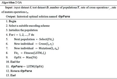
Fig.10 GA steps

The input of the GA is the input dataset, test dataset, number of populations, rate of cross-operation, and rate of mutate operation. The output is the historical optimal solution OpPara and the specific algorithm flow is as follows.

1) Suitable encoding scheme selection. Unlike traditional GAs that use binary encoding, each individual is a one-dimensional array consisting of individual parameters, andnindividuals form a population.

2) Population initialization. Twenty populations are selected using repeated random sampling for population initialization.

3) Fitness value of each individual calculation in the population. The higher the fitness value, the higher the probability of being selected as the final network parameter, indicating that the individual is more genetically competitive.

4) Crossover and variation. The individual genes, i.e., parameters, are crossed and mutated in two with a certain probability, and the number of neurons is affected by the crossover mutation of layers.

5) SETP3-SETP5 repetition. Repeat these steps until the number of iterations reaches the specified number or the fitness reaches the specified value.

6) Individual selection. Select the individual with the highest fitness as the optimal solution to the problem, in other words, the set of LSTM network parameters with the highest recall. The optimal solution is the output to the LSTM network and verified.

The parameters corresponding to the optimal fitness are finally obtained and used as the result of the parameter setting for the model.

3 Analysis of Experimental Results

3.1 Evaluation indicators

In this paper, we use precision, recall, and receiver operating characteristic (ROC) curves[21]as metrics for evaluation. The confusion matrix describes how our model is confused in making predictions. By obtaining the confusion matrix, we can obtain the values of positive samples where the pump is predicted as normal by the model (CTP), faulty samples where the pump is predicted as normal by the model (CFP), positive samples where the pump is predicted as faulty by the model (CFN), and faulty samples where the pump is predicted as faulty by the model (CTN). Generally speaking, the higher the accuracy and recall, the better the classifier. The calculation formulae are

(10)

(11)

whereEaccis the prediction accuracy;Erecis the prediction recall.

ROC is a probabilistic model for comparing the true positive rate (TPR) with the false positive rate (FPR) at different thresholds. In the ROC curve, they-axis is the TPR and thex-axis is the FPR. The ideal effect of the ROC curve is to maximize the TPR while minimizing the FPR.

(12)

(13)

whereRTPRis the ratio of the number of faulty samples predicted to be faulty to the actual number of faulty samples;RFPRis the ratio of the number of normal samples predicted to be faulty to the actual number of normal samples.

3.2 Parameter-optimized LSTM for enhanced models

The deep LSTM network structure can handle massive and complex data in device sensors, but the number of fully connected layers, the number of stacked LSTM layers, and the number of neurons are all important factors that affect the training effect of the network. The optimal parameters need to be chosen to achieve the best training effect. To optimize the parameters of the enhanced LSTM recurrent neural network in this paper, we validated the GA for fine-tuning the parameters of the LSTM for anomaly prediction.

Each individual is initialized to correspond to a set of network parameters of the LSTM model, and each parameter corresponds to a gene in the individual. For example, an individual is (1, 2, 95, 227, 56), where the first three parameters respectively represent the number of LSTM layers, the number of fully connected layers, and the number of neurons in one LSTM layer; the last two parameters represent the number of neurons in two fully connected layers. The range of LSTM layers and fully connected layers is 1 to 3, the number of neurons is between 32 and 256, and eight genes on each chromosome do not reach the length requirement after complementary zeros. The initialization parameters of the GA optimization include the number of populations of 20, the crossover rate of 0.5, the variation rate of 0.01, and the number of iterations of 25. In each training round, the parameters obtained in this round and the size of the fitness are recorded. The number of generations optimized by the GA is 25, and the data for each generation are shown in Table 1.

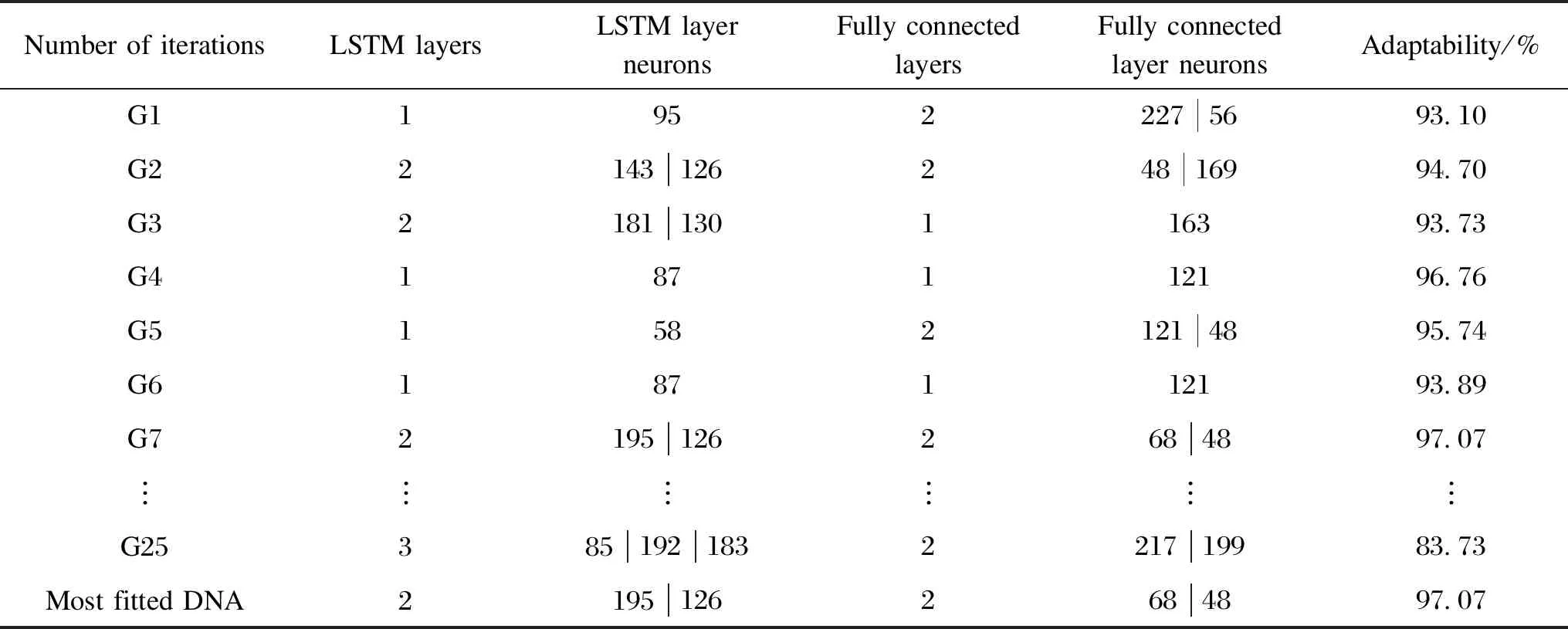
Table 1 Network parameters with the highest adaptability for each generation

The parameters corresponding to the optimal fitness are finally obtained and used as the results of the parameter setting of the model. According to Table 1, the final values of the network parameters were set to the number of LSTM layers as 2, and the number of neurons in LSTM layers as 195 and 126, respectively. The number of fully connected layers was 2, and their corresponding number of neurons was 68 and 48, and the recall rate corresponding to this set of parameters was 97.07%, which was the highest among all generations. The enhanced stacked LSTM network model improved by the GA is shown in Fig.11.

3.3 Accuracy and recall analysis of anomaly detection

Figure 12 shows the accuracy and recall of the algorithm plain Bayesian (NB), recurrent neural networks (RNN), LSTM, and bi-directional LSTM (BiLSTM) after dimensionality reduction. The experimental results show that the network training accuracy and recall of LSTM are 93.56% and 92.45%, respectively, which outperformed the NB, RNN and BiLSTM networks. It has 16.50% higher accuracy and 13.95% higher recall than NB; 1.41% higher accuracy and 2.43% higher recall than RNN; 0.42% higher accuracy and 0.58% higher recall than BiLSTM. It indicates that the LSTM network is superior to the NB, RNN and BiLSTM networks for the processing of pump sensor timing data.

After PCA dimensionality reduction, the accuracy of all three algorithms for pump anomaly detection was reduced to different degrees, but the efficiency was improved. Figure 12 shows the combined results of several experiments. Compared with the LSTM, the accuracy and recall of the PCA-LSTM decrease 1.50% and 2.44%,respectively. In terms of training time, the training results are shown in Fig.13. There is a significant improvement in efficiency. An average of 24 s is saved after dimensionality reduction, indicating the superiority of dimensionality reduction on efficiency improvement.

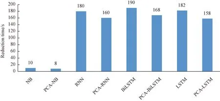
Fig.13 Average dimensionality reduction time of multi-class algorithms

Table 2 shows the accuracy and recall of different algorithms after the GA improvement. The experimental results show that the improved algorithm has a higher accuracy and a better prediction based on the LSTM model, with an accuracy of 96.75% and a recall of 97.07% which are 3.19% and 4.62% higher than those of the original LSTM, respectively.

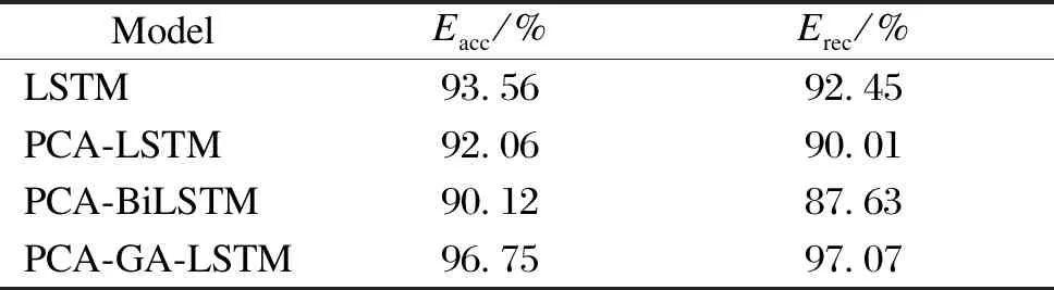
Table 2 Effect of different algorithms after the GA improvement

3.4 ROC curve analysis

The ROC curves of the original process after dimensionality reduction and after GA improvement are shown in Fig.14. Figure 14(a) shows the ROC curve under the original model. The data analysis results indicate that the training accuracy is higher due to the advantage of LSTM’s good processing of time series data. Therefore, LSTM has a larger area under curve (AUC) and better results compared with RNN and NB.

Figure 14(b) shows the ROC curves after parameter optimization by GA, and the data results indicate that the AUC has improved significantly due to the adjustment of the network structure parameters, and the AUC values of the LSTM algorithm are 0.08 higher than that after dimensionality reduction and 0.05 higher than that of the original LSTM, respectively. It represents that the GA has a good effect on our enhanced stacked LSTM network model.

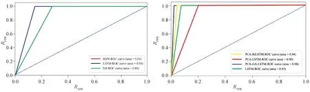
Fig.14 ROC curve results of different algorithms: (a) ROC curves from original model; (b) ROC curves after parameter optimization

4 Conclusions

In this paper, an enhanced stacked LSTM network algorithm for device anomaly detection using sensor data on the device is proposed. The algorithm first extracts the strongly correlated variable data from the sensor data using principal component analysis, realizes the dimensionality reduction of the sensor data, performs anomaly prediction on the reduced dimensional data by augmented stacked LSTM neural network, and uses the GA to optimize the parameters of the augmented stacked LSTM neural network. The experimental validation results conducted by the actual pump real sensor timing data show that compared with the traditional plain Bayesian algorithm with RNN algorithm and the basic LSTM algorithm, the algorithm proposed in this paper has significantly improved accuracy and detection efficiency, which provides a valuable reference solution for anomaly detection of production equipment.

In the future, we will focus on changing the generality of the algorithm, exploring the types of production equipment faults, and performing more refined fault prediction under different anomalies for a more robust equipment fault detection scheme.