TSKARNA-norm Adaption Based NLMS with Optimized Fractional Order PID Controller Gains for Voltage Power Quality

, .

(Department of Electrical Engineering,Sardar Vallabhbhai National Institute of Technology,Surat 395007,India)

Abstract: The operation of a dynamic voltage restorer (DVR) is studied using a three-phase voltage source converter (VSC)-based topology to alleviate voltage anomalies from a polluted supply voltage.The control algorithm used included two components.The first is an adaptive Takagi-Sugeno-Kang (TSK)-based adaptive reweighted L1 norm adaption-based normalized least mean square(TSK-ARNA-NLMS) unit,which is proposed for the extraction of fundamental active and reactive components from the non-ideal supply and is further employed to generate the load reference voltage and switching pulse for the VSC.The step size was evaluated using the proposed TSK-ARNA-NLMS controller,and the TSK unit was optimized by integration with the marine predator algorithm(MPA) for a faster convergence rate.The second,a fractional-order PID controller (FOPID),was employed for AC-and DC-link voltage regulation and was approximated using the Oustaloup technique.The FOPID (PI γD)μ provides more freedom for tuning the settling time,rise time,and overshoot.The FOPID coefficients (Ki,Kd,Kp,γ,and µ) were optimized by employing an advanced ant lion optimization (ALO) meta-heuristics technique to minimize the performance index,namely,the integral time absolute error(ITAE) and assess the accuracy of controllers.The DVR performance was validated under dynamic-and steady-state conditions.

Keywords: Takagi-Sugeno-Kang (TSK),ARNA-NLMS,FOPID-ALO,unbalances,gain optimization,approximation Oustaloup technique

1 Introduction1

Recent advancements in solid-state technologies have led towards comfortable and peaceful lives.These solid-state devices cause power quality (PQ) issues in distribution networks (DNs)[1].PQ issues are exponentially increasing owing to the rapid inventions and applications of sophisticated equipment based on solid-state devices or loads.Recently,researchers have focused on the mitigation of PQ issues,especially voltage related issues,such as sag,swell,imbalance,and distortions.These voltage anomalies and harmonic compensation are efficiently addressed using a series filter called a dynamic voltage restorer (DVR)[2].Owing to unexpected system expansions,three-phase four-wire DNs are experiencing significant power quality PQ issues,such as harmonics,the burden of reactive power,and excessive neutral current[3].A DVR is employed to reimburse the voltages,along with a voltage source converter (VSC) at the load side[4].A study on different PQ issues and their mitigation using a DVR[5]showed the fast response of voltage compensators,such as the static series compensator (SSC),and voltage (sag and swell)correctors,such as the DVR.For the DVR operation,a split-capacitor topology based on the VSC was implemented,and a flux-charge model based on a feedback algorithm was employed to minimize the fault ride[6].Jimichi et al.[7]studied the different architectures of a DVR,where series and shunt converters were connected in an adjacent manner,and described different DC capacitor ratings implemented with various topologies.To compensate for this imbalance,a split capacitor with a battery-supported DVR setup was designed and tested using a transformation-based control algorithm[8].Another study[9]implemented a cascade-based multilayer inverter DVR setup that operated at medium voltage without employing an injection transformer.It is based on a self-supported DC bus capacitor,with the major issue of balancing and controlling the voltage of the DC link.

Numerous control schemes have been actively studied for extracting harmonic components from polluted load currents.Instantaneous reactive power theory (IRPT) involves the transformation of voltage and current to compute the active and reactive powers.The drawback is that it becomes difficult to operate under a non-ideal supply voltage[10].The synchronous reference frame theory (SRFT) versatile control technique estimates the DC quantity from three-phase components and realizes harmonics by employing a low-pass filter (LPF)[11].

Adaptive filtering is a well-known control method for estimating the reference sinusoidal component from a disturbed load current.Adaptive filters have numerous applications in signal processing and control engineering.However,adaptive control algorithms offer optimal solutions over classical control approaches,particularly when the load is uncertain,which involves complex systems.The least mean square (LMS) control scheme is often used as an adaptive controller in a DSTATCOM[12].An appropriate step size selection is required to optimize the error,which increases the accuracy and convergence rate.The step size is directly proportional to the convergence rate and inversely proportional to the accuracy,which means that a higher step size value results in faster convergence but leads towards instability.Considering the convergence rate,step size,and control performance,a tradeoff is required to resolve this contradiction while selecting the objective.The contradiction between objectives is solved by selecting an appropriate convergence coefficient[13].Researchers have been interested in improving control setting optimization over the past several years.The frequently used LMS algorithms for improving PQ are normalized-LMS,variable step-size,and leaky LMS[14].Several control algorithms based on step size selection LMS[15]and variable LMS (VLMS)[16]have been recommended.A study[17]illustrated the PQ concerns in distributed generation and mitigation using various custom power devices (CPDs).With the power normalization concept based on the selected input elements,an adaptive family of the LMS,that is,NLMS,was proposed because it offers an optimized solution to select the step size and resolve the stability issues of the classical LMS[18].Other methods,such as the fuzzy-inference-based LMS[19]and Kalman filter,have complex implementations in real time.The aforementioned methods include the adaptive filter theory.The adaptive technique estimates filter coefficients by optimizing the errors.The key drawback of the classical LMS is its early convergence.The proposed Takagi-Sugeno-Kang (TSK)-based adaptive reweightedL1norm adaption-based NLMS(TSK-ARNA-NLMS) belongs to an extended family of the ZA-LMS,and its control scheme is simpler than that of the LMS in terms of computational complexity,but it is relatively complex to analyze.

The DVR control is combined with two fractional-order PID (FOPID) controllers for DC-and AC-link voltage stabilization and regulation.The FOPID has more flexibility in tuning the system coefficients than the classical PID controller owing to its five degrees of freedom.The benefits of implementing the FOPID include less overshoot,low oscillations,and robustness against disturbances.Tuning of the FOPID controller coefficients is a challenging task; therefore,metaheuristic techniques such as BBO[20],particle swarm optimization (PSO),genetic algorithm (GA)[21],and artificial bee colony(ABC)[22]have been employed for FOPID coefficient tuning.This reduces the computational effort and error,with a better response to the time characteristics.The optimal coefficient of the FOPID was obtained using the integral time absolute error (ITAE) as a performance index.The aforementioned metaheuristic techniques have the disadvantages of local stagnation,premature convergence,difficulty in choosing controller coefficients,and extended computational time[23].Therefore,parameter settings are made using an advanced algorithm,namely,the ant lion optimization (ALO)-based FOPID,which converges around the optima and has fewer algorithm-specific parameters to obtain the gain coefficients in less evaluation time.It also avoids local entrapment and achieves an objective function by optimizing the search space[24].

In this study,a TSK-ARNA-based NLMS with three single-phase VSC-based control strategies was recommended.The main motivation for using unipolar modulation instead of bipolar switching is to reduce switching losses because it has a lower switching frequency and low-voltage ripples than bipolar switching.The proposed TSK-based ARNA-NLMS control scheme was developed to update and select the optimal step-size coefficient.This resolves the conflict between convergence rate and stability by determining the step size using the marine predator algorithm(MPA) heuristic method.The advantages of integrating the MPA into the proposed control algorithms are self-adjustment to improve the tracking capability,robustness against system parametric variation,and improved response under a dynamic state.The control algorithm achieved a faster convergence response with fewer static errors.The DC-and AC-link voltages were maintained constant at the set values using the FOPID-ALO control.The FOPID gains were estimated using the ALO optimization technique.Finally,the TSK-ARNA-NLMS controller evaluated the gate signal using the generated reference load voltage component.Simulation and hardware results confirmed the effectiveness of the proposed control scheme.The main contributions of this study are as follows.

(1) A 3-single phase VSC-based DVR topology was proposed for the restoration of load voltage under a highly polluted supply voltage.

(2) The trained TSK-ARNA-NLMS model accelerated the computation of the direct and quadrature weight components and leveraged the MPA to obtain the optimal step size.The forecasted optimized results were evaluated using statistical criteria.

(3) A FOPID was proposed,whose coefficients were optimized by the ALO to maintain a constant AC-and DC-link voltage at the PCC.The accuracy was measured using a performance index (ITAE).

2 System layout description

The 3P4W DVR configuration is shown in Fig.1.The presented configuration provides the complete details of the main components connected to the DVR topology.A non sinusoidal supply voltage is introduced to represent all electrical voltage disturbances (sag,swell,imbalance,and distortion).The connected sensitive load was modeled using a combination of resistive (RL) and inductive (LL)elements.The interfacing inductor (Lf) is used to filter out the ripples,and the VSC is connected through (Lf)at the PCC[4].On the other side of the PCC,an RC filter (Rf,Cf) is provided to suppress the ripples in the voltage[5,7].

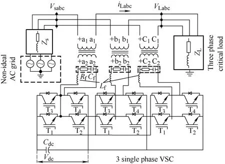
Fig.1 Schematic of the proposed DVR

3 Control methodology

The key purpose of proposing the TSK-ARNA-NLMS controller is to resolve the contradiction between step size and convergence rate.The stability and convergence rate depend on the step size[1,14-15].The step size,λ(z) depends on the operating coefficients and should be adaptively updated with the loading and dynamics present in the system to achieve a better tracking performance of the filter.Therefore,the step size needs to be automatically adjusted using the TSK unit and is optimized using the MPA technique to obtain the optimal FIS to reduce the error.This improves the estimation process for extracting the fundamental quantity from a non sinusoidal supply.The estimated fundamental components were averaged to obtain the values for the direct and quadrature units.The load voltagein reference was obtained by taking the product of the load current template with the in-phase and quadrature unit vectors.The FOPID(PIγDy) coefficients were tuned using the ALO technique to control the DC and AC-link voltages.The subsequent gate pulse for the VSC was generated by processing the extracted error via pulse-width modulation (PWM).The complete TSK-ARNANLMS with FOPID-ALO control is shown in Fig.2.A detailed description of the mathematical formulation is provided in the following section.

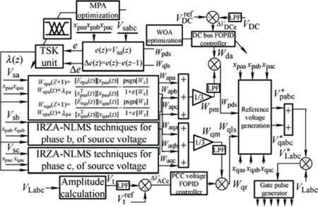
Fig.2 Control architecture of combined TSK-ARNA-NLMS algorithm

3.1 Extraction of fundamental weight components of active power

Initially,the fundamental component extraction was derived using the active unit template components (xpaa,xpab,andxpac) for the three phases,where the magnitude of the load current (ilp) is computed as follows

The unit template in-phase componentx(z) is computed as

Electrical voltage disturbances,such as imbalance or distortion,are caused by positive,negative,and zero sequences,along with harmonic components in a three-phase system[21-22].

The components of Eq.(4) represent the positive,negative,and zero sequences,respectively,denoted by the subscripts+,-,and 0.The fundamental components of the system voltage frequency are the positive,negative,and zero sequences.

Normally,the voltage at the load terminal is expected to be sinusoidal with set amplitudeVl.

Hence,series-based converters must compensate for the following components.

The TSK-ARNA-NLMS control algorithm determines the fundamental weight quantity of the active and reactive from the non-sinusoidal input voltage at thezthsample,which is computed as

Periodic and disturbed voltages can be expressed by the algebraic summation of the fundamental quantity of frequency and multiple quantities of the fundamental frequency.

The voltage corresponding to the fundamental and harmonic components of the supply voltage can be expressed as

whereωrepresents the frequency of theqthcomponent,aq=Vsfcosφq,bq=Vsfsinφq.Then,Eq.(10) can be written as

TheVsfcosφf,Vsfsinφf,Vshcosφf,andVshsinφfterms are replaced withwa1,wb1,wah,andwbh.The new equations can be written as follows

where ‘h’ represents the order of the harmonic.The estimated grid voltage is computed from the optimal weight values (wa1,wb1,wah,andwbh),and is expressed as

wherex(z) is the input vector and is represented asx(z)=[sinωzcosωzsin5ωzcos5ωz…]T,which represents the unit template of the in-phase and quadrature components,[ypayqay5pay5qa]T.The unit quadrature vector components are described in the following subsection.The weight vectorwTis defined as follows

The errorErpa(z) between the actual source voltage and the estimated voltage component is computed as

The cost function of MSEε[E2rpa(z)] is minimized by optimal weight selection.These weights are continuously optimized by the proposed TSK adaptive reweightedL1norm adaption-based LMS control algorithm and are estimated at the (z+1)thinstant expressed in Eq.(18)

L1norm with respect to ‘w’

3.2 TSK acclimation and development of a Sugeno model based on the marine predator algorithm

The proposed TSK unit is a multilayer network,and no defuzzification is required to obtain the output response.Circle and square nodes were incorporated into the network to reflect the adaptive behavior of the model.The input-output data sets were mapped by employing triangular and trapezoidal membership functions (MFs),and their behavior depended on specific components.The main task was to automatically tune the MFs to adapt to uncertain variations in the system and achieve an optimal FIS.This is obtained using MPA learning,which avoids the arbitrary selection of MFs that alters the accuracy of the target’s response.The TSK unit was fed with two input signals,represented as

The detailed layer-wise function is as follows.

Layer 1 feeds two inputsx1andx2and each input is assigned three MFs.The nodes or MFs are designated as square brackets and their internal control structures are represented by trapezoidal and triangular MFs.This process is called fuzzification,and the equations used to represent each MF are Eq.(20).

Layer 2 multiplies the incoming voltage signals at each node and follows the fuzzy rules.Each node forwards the output resulting from the next node and has weightsW1andW2.

Layer 3 collects the training dataset from the controller and implements the learning algorithm.This includes the detection and correction of errors during training.

where {mi,ni} are parameter sets andi=1,2,and 3.These antecedent parameters {mi,ni} change the error value and desired linguistic variables created for each selected MF.

Layer 4 involves the defuzzification process,and the following parameters are used to derive the inference rule

whereb01,b02andr1are the consequence parameters.As a result of the learned neurons being inserted into Layer 5,an optimal output is produced as the desired signal.Consequently,the TSK model supervises the absolute control strategy.

The overall output signal from TSK optimization begins with the initial assigned random weight value and is continuously updated under an iterative process.The updated weight vector changes the value function estimated using the collected training dataset.Finally,the summing node evaluates the deterministic value in terms of the positive and negative weighted neurons in the interconnected layer.Possible linguistic rules are listed in Tab.1.The inference engine system incorporates these rules to achieve the required target output.The proposed TSK unit was employed to evaluate the step sizeλ(z) and determine the optimal weight required for the ARNA-LMS algorithm to reduce error.The convergence curve of TSK for step size selection ‘λ’ is depicted in Fig.3.The fuzzy subset for inputs e and Δe is determined using three variables(NB,Z,and PB) and 3×3=9 rules to emphasize the capability of the TSK controller.Tab.2 describes the performance evaluation tools for the TSK unit used for step size tuning.

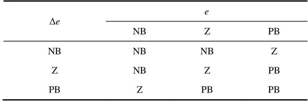
Tab.1 Rule base with 9 rules

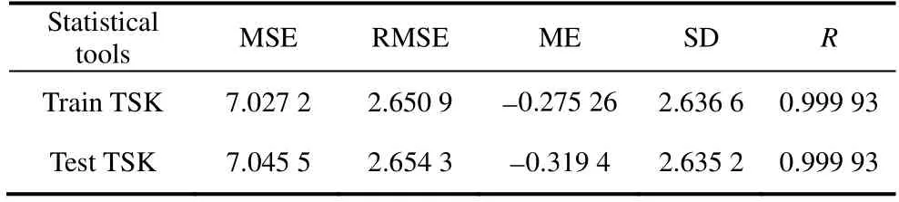
Tab.2 Statistical performance tools of TSK unit for step size (λ) selection

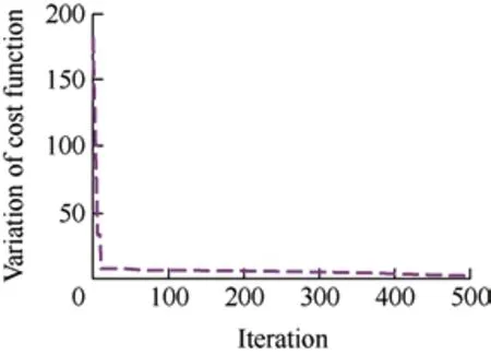
Fig.3 Convergence curve of TSK for step size selection ‘λ’

3.3 Implementation of MPA-TSK optimization

The error signale(z) was optimized by learning the antecedent and consequence parameters of the TSK unit using the MPA technique.Statistical metrics,namely,mean square error (MSE),root mean square error (RMSE),standard deviation (SD),mean error(ME),and coefficients of correlation (R),were considered to investigate the accuracy of the prediction results of the TSK-MPA.The MPA is mainly inspired by the foraging mechanism of predators in the ocean and simulates this mechanism by employing Levy-and Brownian-based movements between the predator and prey.These are adopted by ocean predators to determine the optimal foraging in terms of the FIS parameter of the TKS unit.The step sizeλ(z) was computed using the TSK structure based on the ARNA-LMS method expressed in Eq.(20).This estimates the active fundamental component for phase ‘a’ at the (Z+1)thinstant.It is estimated as

Similarly,active components for phase ‘b’ and phase ‘c’ are represented as

whereErpa,Erpb,andErpcrepresent the actual components of the error vectors of phases a,b,and c,respectively,for the recommended TSK-ARNANLMS-based controller.The mean output value corresponding to the fundamental active power weight components is computed using Eqs.(25)-(27).

Similarly,the reactive power weight components extracted for phases a,b,and c were computed as follows

wherexqaa,xqab,andxqacare quadrature components computed using Eq.(32).

Because the weights are adaptive,they are updated continuously.Therefore,a precise value is obtained by taking the average value of each phase of the reactive weight (wqm),which is evaluated as

4 FOPID controller-based voltage regulation

A significant improvement in the voltage at the DC and AC buses is achieved by maintaining the voltage fluctuations within an acceptable level if the actual voltage value is kept closer to the set value.This minimizes the error level by implementing the intelligent FOPID integrated with ALO.The ALO meta-algorithm reduces the computational effort required for fine-tuning to achieve optimal coefficients,and it accurately determines the active and reactive estimated load components.

The FOPID controller is operated by feeding error components (VDCe) and regulates the voltage error to enhance tracking to reach to the reference level.The error values of the DC-link voltage are expressed as follows

Prior to Holly s birthday, Susan had been a regular visitor in our home. On several occasions, she rode the bus home with Holly and was one of the few friends ever permitted to stay over on a school night. The girls did their homework together and went to bed at a reasonable hour.

The FOPID controller response (daw) is subtracted from the mean of the direct component (wpm) to obtain the desired active fundamental (wpds),as shown in Eq.(35).

The terminal voltage (Vt) is computed using Eq.(37)and compared with the reference value (Vtref).The estimated error values are used as inputs to the FOPID to maintain the desired voltage.

The outcome of the FOPID (wqr) is the sum of the quadrature mean value (wqm) required to achieve the desired quadrature fundamental quantity (wqls),as shown in Eq.(38).

The template vectors in Eqs.(2) and (32) are implemented to estimate the reference direct and quadrature elements.

The termsWpdsandWqlsare the adaptive direct and quadrature quantities,respectively.These weights are used to determine the reference quantity of the load-side voltage.The reference load voltage is derived using Eq.(40).

4.1 FOPID controller approximation and its gains optimization using ALO

The FOPID is employed as the DC and AC bus voltage regulator for the proposed system.The FOPID control is an extended-family member of classical PID controllers.This control mechanism has five degrees of freedom (Ki,Kd,Kp,γ,andµ) and therefore,compared with the classical PID controller,this feature offers more flexibility and robustness in the tuning of FOPID coefficients by employing the fractional calculus[20].The mathematical time-domain representation of the FOPID controller can be defined as

The Laplace form of Eq.(41) is obtained as

whereKdenotes the adjustable transient gain.Mis the approximation order.wzmandwpmdenote the approximated frequencies of the poles and zeros,respectively,and their values lie in the interval of thewl(lower) andwh(higher) transitional frequency fitting range.Here,ALO optimization is integrated with the FOPID controller to fine-tune the coefficients,which accelerates the time-response characteristics of the systems in terms of rise time (tr),settling time (ts),and overshoot (Mp).

4.2 ITAE as an objective function

The ITAE evaluation metric was used to measure the performance of the designed ALO-FOPID controller.

where,,andrepresents the lower values,,,andindicates the upper values of the controller parameters.,,,andare the lower and upper range values of integral and derivative order.

4.3 Implementation of ALO-FOPID gain optimization

The control parameters (Kp,Ki,Kd,γ,µ) are tuned by minimizing the selected performance index (ITAE).To optimize the controller and gain values,the ALO technique was employed to obtain the optimal values of the FOPID.The proposed ALO is summarized in the following five steps that describe the hunting strategy of the antlion: ① randomized walking of ants,② building the traps,③ entrapping of ants,④catching prey,and ⑤ rebuilding the traps for hunting.Detailed mathematical modeling of the hunting behavior and entrapment is described in reference[29].The gain tuning of the FOPID coefficients using ALO is illustrated in the block diagram in Fig.4.The ALO was employed for FOPID gain tuning,and the error quantity was used to derive the cost function defined in Eq.(45).The basic ALO equations are based on ant and ant lion behaviors.Random walk was selected to model the ant motion and search for food based on stochastic movement.

wherekrepresents the random stroll,cumsumdenotes the cumulative sum,nis the max iterations,r(k) is the stochastic,and

where ‘rand’ represents the randomly generated number in the interval [0,1].The locations of the ant(A) and antlion (Ak) were modeled using the matricesMantandMantlion,respectively.The termsAi,jandAki,jrepresent the location ofithant and antlion,respectively,in thejthdimension.

wherei=1,2,…,n/m,j=1,2,…,d,nis the ant number,mis the antlion number,anddis the dimension of the variables considered.The cost functions defined in Eqs.(49)-(50) was used to evaluate the fitness at each iteration of the optimization process.The termsMFitaandMFitalare the matrix representations of each ant and antlion for saving the cost function,respectively,and are expressed as

The mathematical modeling with boundaries for random search space is given as

A roulette wheel was used to select the optimum antlion.Complete entrapment is performed by the antlion,which slides the sand to the pit center when it realizes that the ant is in a trap or pit and tries to escape from the trap.This trapping is performed by throwing the sand into the pit using its mouths,and this mechanism leads to the reduction of the ratio pit,as expressed by Eq.(53).

Here,M=10w×(k/),wherekis the current iteration,lis the total number of iterations,andwis an iteration-dependent constant.The final stage of hunting the prey is mathematically expressed as Eq.(54)

Here,antlion eats the ant when an ant is a fitter compared to antlions means ants are trapped by pulling the sand into the pit.This equation indicates that the new location of the antlion was updated for the next hunt.During the optimization process for finding the coefficients of the FOPID controller,the parameter values considered are as follows: population size is equal to 12,maximum trials are 50,and total number of variables equal to 10 (Kp1,Ki1,KD1,γ1,μ1andKp2,Ki2,KD2,γ2,μ2i).The tuning performance of the FOPID controller is illustrated in Fig.5.Fig.5a shows that the ALO-FOPID cost function converges to 43.233.Figs.5b-5f depict the performance characteristics for the estimation of the FOPID controller gain coefficients.The recorded and converged responses of the DC-link voltage with the tuned value of the FOPID controller gain coefficient obtained using a trial-and-error approach are listed in Tab.3.The estimated value of the FOPID using ALO outperformed the others,and it was observed that the error regulation was better for DC-link voltage.Similarly,the AC-FOPID controller gain coefficient (Ki2,Kd2,Kp2,γ2,andµ2) variations against iterations are presented in Tab.3.

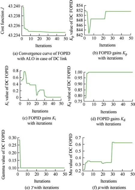
Fig.5 Tuning performance of FOPID controller

4.4 Reference estimation and gate pulses

The required load quantity of the reference voltage(V*Labc) was evaluated by summing the direct (V*pabc)and quadrature (V*qabc) reference components

The switching signals for the three-phase VSC were evaluated by processing the errors generated by comparing the reference value of load voltage (V*Labc)with the actual measured load voltage (VLabc).

5 Results and discussions

The Matlab environment was employed for the integrated TSK-ARNA-LMS control algorithm of a 3 single-phase DVR system.The DVR model was simulated using a sampling time (ts) of 20 µs.The optimized TSK-ARNA-NLMS-based controller was corroborated under all considered voltage imperfections in the grid.The performance was analyzed by employing the DVR compensator and explained using the simulation and experimental responses.

5.1 Voltage disturbance compensation capability of DVR using RNA-NLMS-based algorithm

All of the aforementioned voltage concerns in the supply voltage are considered when analyzing the overall DVR effectiveness in Fig.6.The supply voltage (vs) is shown in Fig.6a with disturbances such as voltage sag,swelling,distortions,and unbalances.The subplots (2)-(4) represent the three-phase compensation voltages (Vca),(Vcb),and (Vcc),respectively.Subplot (5) presents the sinusoidal and balanced load currents (iLabc).Subplot (6) in Fig.6a represents the constant load voltage (Vlabc) irrespective of imperfections in the supply.The wave signals of the DC-link (Vdc) and AC-link voltages (Vt) are shown in subplots (7) and (8) of Fig.6a.From Fig.6a,it is observed that the magnitudes of the terminal voltage (Vt) and DC-link voltage (VDC) are retained at their set levels,even during dynamic scenarios.Fig.6a shows that the integrated TSK-ARNA-NLMS-based control effectively compensates for the above-mentioned voltage PQ electrical disturbances created in the supply voltage,and the corresponding load voltage reaches the required level.Fig.6b illustrates the DVR response during the voltage-imbalance state of the supply voltage.Here the learning rate is selected by the TKS optimized unit and shows that the DVR takes 0.03 s for compensating the voltage imbalance from the supply.

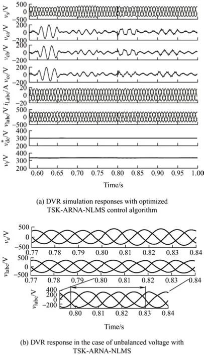
Fig.6 Compensation of voltage-based power quality problem

5.2 Power quality harmonics analysis of DVR under distorted supply voltage

The injected harmonics is analyzed for phase ‘a’ in the supply voltage which helps to retain the harmonics at load under an acceptable limit of 5%.

Thus,the spectral analysis of the distortions in the case of the supply (vs) and load voltage components(vl) is depicted under a steady scenario.Fig.7 shows the load voltage THD after compensation with the optimized TSK-ARNA-NLMS control; its value is 3.93%.Tab.4 and Fig.8 provide a detailed comparative analysis of the DC link behavior after evaluating the dynamic performance indicators,such as the rise and settling times with overshoot.The statistical values are listed in Tab.4 and Fig.8.The performance indices confirm that the proposed TKS-ARNA-LMS requires less time to stabilize with small oscillations and prove its performance effectiveness and efficacy.

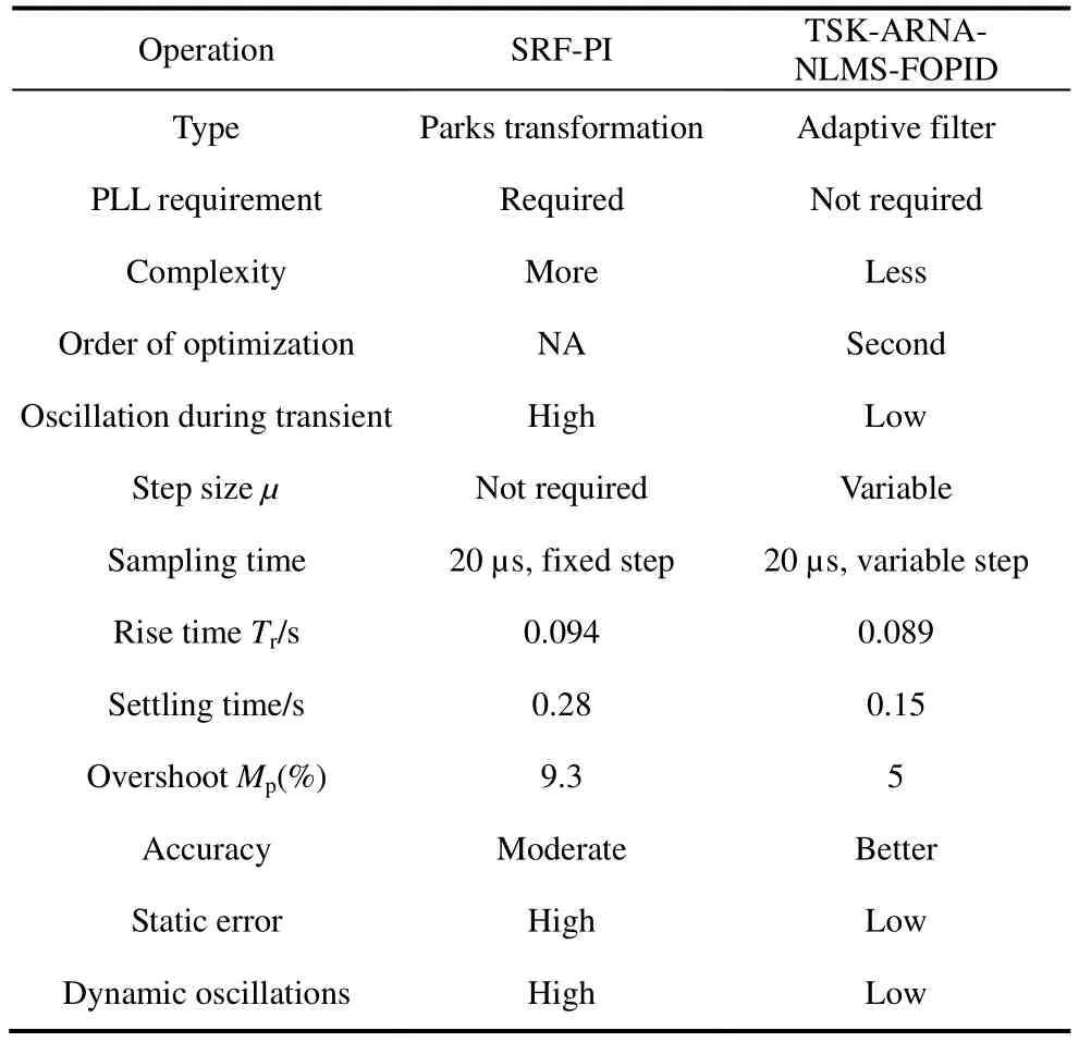
Tab.4 Comparative performance of the TSK-ARNA-NLMS-BASED algorithm with SRF-PI

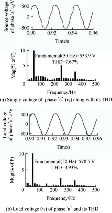
Fig.7 Harmonics FFT during voltage distortions in supply-side voltage

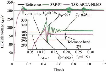
Fig.8 Dynamics of DC-link voltage using SRF-PI and TSK-ARNA-NLMS-FOPID

6 Experimental performance

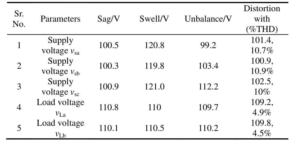
The proposed TSK-ARNA-NLMS-based DVR control algorithm was corroborated by its steady-state and dynamic nature.Using a d-SPACE-based Micro Lab Box CPU,a prototype with scaled-down factors was evaluated in the laboratory at sampling time (ts) equal to 40 µs to measure the accuracy of DVR with the considered PQ concerns.The dynamic results were captured with a DSOX2004A,which is four-channel-based.Fluke-43B was employed to save the results of the voltage imbalance and distortion under steady-state conditions.These experimental results were presented using a DSO display window,with half of them shown in a normal working state and the other half in a dynamic state with voltage-related PQ concerns.The simulation and experimental data are provided in Appendix A and B.

6.1 Experimental extensive internal control signal response

The TSK-ARNA-NLMS-based control signals are shown in Fig.9.The reference load voltage is derived at PQ events in the grid for ‘a’ phase.Fig.9a includes the signals of phase ‘a’: supply side like supply voltage (vsa),unit weight vector of direct quantity (upa),actual computed error (ea),and the TSK-ARNANLMS term,denoted byλTSK-ARNA-NMLS,which is employed in the direct weight updating under distortion state.The fundamental direct quantity (Wspa),mean fundamental direct quantity (Wpm),maintained and stabilized DC voltage (Wda) responses,and total direct weight (Wpds) are shown in Fig.9b.

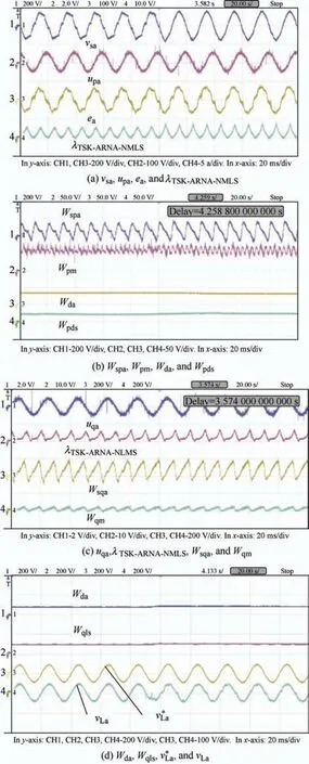
Fig.9 Internal signals of the TSK-ARNA-NLMS-based controller for phase ‘a’ of distortion PQ event in supply

Similarly,for the reactive quantity,Fig.9c presents the phase ‘a’ response,which includes the quadrature vector (uqa) and the TSK-ARNA-NLMS term,denoted byλTSK-ARNA-NMLS,which help in the reactive weight updating,with the fundamental quadrature quantity(Wsqa) and mean reactive weight (Wqm); these are described with the dynamics during a case of distortion.The effectiveness of the control scheme is illustrated by the tracking ability of the load voltage,even at voltage imperfections in the supply,as shown in Fig.9d.The captured waveforms show the outcome of the AC-bus voltage (Wqr),total quadrature weight(Wqls),and reference computed load-end voltage (v*La)effectively tracked with the actual measured load-side voltage (vLa).

6.2 Experimental DVR results with proposed methodology TSK-ARNA-NLMS

Fig.10 shows the compensation achieved by employing the TSK-ARNA-NLMS in the case of a voltage swell.The signals illustrated in Fig.10a are voltage swells in the supply (vsabc) and the restored 110 V RMS with a balanced voltage (vLabc) at the load.

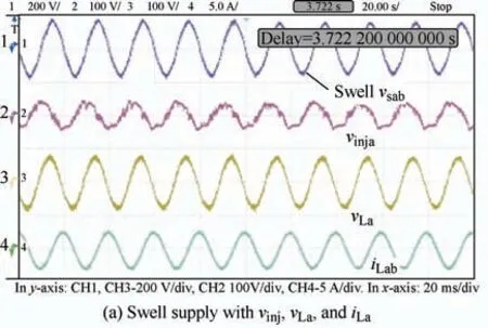
Fig.10 Compensation behavior

6.3 Steady state performance

The steady-state results under sag and distortion are shown in Fig.11 and their statistical values are listed in Tab.5 for a detailed analysis.A sag of-10% that is injected intovsis shown in Fig.11a,and the restoration ofvlafter compensating for the voltage disturbances is demonstrated in Figs.11b and 11e.Figs.11c and 11d show the harmonics injected intovs,and Fig.11f shows that the fundamental was efficiently filtered to 4.9%.

Tab.5 Experimental statistical values for steady state

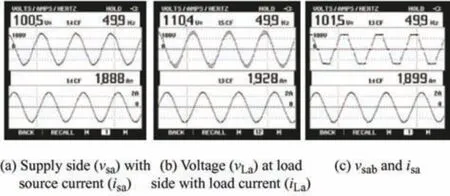
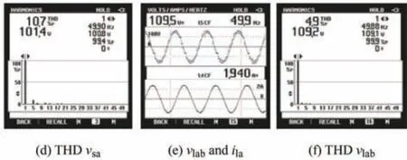
Fig.11 Performance experimental response under sag

7 Conclusions

This paper presents the implementation of an optimized TSK-ARNA-NLMS-based DVR control scheme integrated with metaheuristic techniques,namely MPA and ALO.This optimized TSK-ARNA-NLMS controller was developed to extract the fundamental weights from the polluted supply voltage,and the step size was determined by employing a TSK unit that adapts to the changes quickly,and rapidly updates the weight vector.This was used to estimate the reference load-voltage component.The meta-algorithm ALO-integrated FOPID controls the voltage stabilization and dynamics in DC-and AC-link voltage,and this intelligent control reduces the computation efforts required to tune the five coefficients (Ki,Kd,Kp,γandµ) of the FOPID controller.The DVR enhanced the PQ performance and after compensation,the THD in load voltage was within the IEEE-519 limit.Under steady-state and unbalanced load state,the magnitude of voltages at the PCC and DC-link was maintained at their reference set levels.The compensatory time response was investigated under an imbalanced state of voltage and the capability of the DVR was observed in terms of the fast compensation of the voltage disturbance,in 0.03 s.The control experiment on a DVR prototype using d-SPACE showed satisfactory results under both operating states.

Appendix A

Voltage at supplyVL-L=410 V,50 Hz with 15 kV·A load,0.8 p.f; load current (iL)=21.12 A; transformer DVR rating=5 kV·A,200/200 V;VDC=300 V;CDC=1 200 µF; filter/interface inductor (Lf)=1.5 mH;filtering component with 6 Ω of resistance (Rf) and capacitor (Cf) of 10 µF.LPF with a cut of frequency=10 Hz; sample time (ts)=20 µs.

Appendix B

Non-sinusoidal grid supply of 110VL-L,50 Hz with a load of 0.352 kV·A; load current (iL)=2 A;transformer rating for DVR: 4 kV·A,125/125 V;DC-bus voltage (Vdc)=35 V; DC-bus capacitor (Cdc)=4 700 μF; and interface inductor (Lf)=1 mH;components of ripple filter:Rf=10 Ω andCf=120 μF,sample time (ts)=40 μs.The coefficients of the FOPID for the DC link arekp1=0.1,ki1=0.1,kd1=0.1,γ1=0.1 andμ1=0.6.AC link coefficients arekp2=0.1,ki2=0.1,kd2=0.1,γ2=0.8 andμ2=0.8.