Fast Solution Method for the Large-scale Unit Commitment Problem with Long-term Storage*

, , , *, ,

(1.School of Electrical Engineering,Guangxi University,Nanning 530004,China;2.State Grid Sichuan Electric Power Company,Chengdu 610041,China;3.National Power Dispatching and Control Center,State Grid Corporation of China,Beijing 100031,China;4.National Engineering Laboratory for Big Data Analysis and Applications (Peking University),Beijing 100871,China)

Abstract: Long-term storage (LTS) can provide various services to address seasonal fluctuations in variable renewable energy by reducing energy curtailment.However,long-term unit commitment (UC) with LTS involves mixed-integer programming with large-scale coupling constraints between consecutive intervals (state-of-charge (SOC) constraint of LTS,ramping rate,and minimum up/down time constraints of thermal units),resulting in a significant computational burden.Herein,an iterative-based fast solution method is proposed to solve the long-term UC with LTS.First,the UC with coupling constraints is split into several sub problems that can be solved in parallel.Second,the solutions of the sub problems are adjusted to obtain a feasible solution that satisfies the coupling constraints.Third,a decoupling method for long-term time-series coupling constraints is proposed to determine the global optimization of the SOC of the LTS.The price-arbitrage model of the LTS determines the SOC boundary of the LTS for each sub problem.Finally,the sub problem with the SOC boundary of the LTS is iteratively solved independently.The proposed method was verified using a modified IEEE 24-bus system.The results showed that the computation time of the unit combination problem can be reduced by 97.8%,with a relative error of 3.62%.

Keywords: Constraint splitting,long-term storage,mix-integer programming,unit commitment

1 Introduction1

Unit commitment (UC) with various security constraints is a key tool for simulating the unit dispatch of various generators in power system optimization,the electricity market,and generation expansion planning[1-2].Traditional UC is a mixed-integer linear programming problem involving a large amount of 0-1 variables indicating the on/off states of thermal units and coupling interval constraints (ramp rate constraints and minimum up/down time constraints)[2].When incorporating the high penetration of renewable energy sources such as wind and solar power,short-term storage is an effective technology for addressing the diurnal fluctuations in variable renewable energy (VRE)[3-4].However,seasonal fluctuations over multiple weeks or months require long-term storage technologies to shift energy over long periods[5].Beyond diurnal storage,research has observed that storage technologies with an even longer duration (> 12 h) can support the integration of high penetration of VRE by shifting energy during multi-day periods of supply and demand imbalances.Several candidate long-term storage (LTS)technologies are available,such as pumped hydro,hydrogen,and compressed air energy storage[6].

Although many efforts have been made for the technical and economic assessment of LTS[7-8],a key limitation lies in modeling long-term storage in UC.Generally,UC with short-term storage is solved by selecting representative periods or decomposing the problem into several minor sequential problems[9-10].In contrast,UC with long-term storage must consider inter-period arbitrage,thereby increasing the computational burden owing to the coupling constraints of long-term storage,particularly the state of charge constraint.

Four main methods are used to address the above problems ① scenario-based method[10-11],② piecewise sequential method,③ Lagrangian relaxation (LR) based method,and ④ parallel horizon-splitting method.For scenario-based methods,representative days are selected based on temporal clustering algorithms,such as k-means[12],k-medoid[13],and hierarchical clustering algorithms[14].Nevertheless,typical periods are independent and cannot exchange energy,leading to deviations in the results and underestimation of the value of seasonal storage when incorporating a high share of renewable energy[15].Ref.[16] proposed a novel seasonal storage model based on inter-period and intra-period states to model the sequential characteristics between typical periods.For the piecewise sequential method,the long-term dispatch problem is decomposed into many smaller problems that are solved sequentially.The final state of the units in each period is restricted to the state of the units of the next period to satisfy the ramp rate constraints and minimum up/down time constraints of the thermal units.In Ref.[17],the entire year of time-series data in the high-resolution test system was separated into 61 individual periods with 144 consecutive hours and run consequently.Although this approach guarantees the feasibility of a solution,its optimality is not guaranteed.For the LR-based method,system-wide constraints are relaxed using the introduced Lagrangian multipliers and solved iteratively until convergence.Ref.[18] developed a surrogate LR method and proved its convergence to optimal multipliers.This method was recently applied to the hourly UC problems in Ref.[19].Ref.[20] proposed a fast solution method for solving the UC problem based on LR and dynamic programming.For the parallel horizon splitting method,the long-term horizon is first split into many small periods,a feasible solution is then by solving each subproblem in parallel,and the feasibility of solutions for the original problem is iteratively validated[21-22].The approach performs well in addressing long-term optimization problems with ramp rate and minimum up/down time constraints on the thermal units.However,this approach fails to include long-term storage technologies whose energy arbitrage over a period is longer than the representative period.

In summary,the above methodology makes it difficult to address the long-term UC problem using LTS.Regarding the operation of renewable-dominated power systems with LTS,focusing on the optimal operation schedule of thermal generators,renewable generators,and LTS to increase renewable energy utilization.LTS is used to shift renewable energy curtailment to the peak period of load demand by optimizing the yearly operation schedule.For the entire charging/discharging optimization problem of LTS to be covered,the schedule horizon should be an entire year.The time-coupling constraints of the state of charge (SOC) of LTS are difficult to decompose owing to a lack of global vision.Obtaining “good enough” solutions for the original UC while improving significantly solving efficiency is necessary.

The motivation of this paper is to propose a fast solution for solving long-term UC with LTS coupled constraints based on time horizon splitting.The main contributions of this paper are as follows.

(1) Based on the time horizon splitting method,the framework and detailed procedure of the bi-level optimization model for UC with time-coupling constraints of LTS are proposed to improve the solving efficiency.The upper-level model solves the UC without LTS using a time-horizon splitting approach to perform a chronological simulation of the power system.The lower-level model solves the price-arbitrage model of the LTS to optimize its yearly operation based on the locational marginal prices(LMPs) from the upper-level model and nodal net load constraints.The lower-level model is used to generate the SOC targets at the end of each sub problem.The upper-level model is then run again with the optimized operation results of the LTS from the price-arbitrage model as constraints for the LTS.

(2) A method for constructing an SOC boundary of the LTS at the end of each sub problem is proposed to decouple the time coupling constraints.Moreover,a method for constructing a feasible solution to the original problem based on the sub problems is proposed to obtain a “good enough” solution compared with the original problem.

The remainder of this paper is organized as follows.The proposed LTS model and UC problem with the LTS is presented in Section 2.The procedure for horizon splitting and solution construction is presented in Section 3.Section 4 also presents the simulation results.Finally,Section 5 concludes the paper by summarizing the results.

2 Mathematical modeling

2.1 Nomenclature

(1) Indices

sIndex of storage

tIndex of period

gIndex of generator

zIndex of node

tkIndex of period for thek-th sub problem

ΨIndex set of generator units

TIndex set of time indices

ΨTIndex set of conventional generator units

ΨRIndex set of renewable source generator units

ΨSIndex set of long-term energy storage units

(2) Variables

Sg,tStarting status binary variable

Dg,tShutdown status binary variable

Ug,tOnline/offline state

Charging power of storagesat periodt

Discharging power of storagesat periodt

Pg,tPower output of generator unitgat periodt

Upward spinning reserve capability of generatorgat periodt

Downward spinning reserve capability of generatorgat periodt

Upward spinning reserve capability of storagesat periodt

Downward spinning reserve capacity of storagesat periodt

NkNumber of sub problems

ag,kPeriods that must be adjusted in the end part ofk-th sub problem

bg,kPeriods that must be adjusted in the beginning part of (k+1)-th sub problem

akMaximum value ofag,k

bkMaximum value ofbg,k

(3) Parameters

ΔtDuration of a period

Net load at periodt

PTDFPower transfer distribution factor matrix

Ss,tState of charge of LTS units at periodt

State of charge of storagesafter supplying reserve at periodt

Dual variable of system-wide power balance constraint

Transmission upper limit

Transmission lower limit

f0(Pg,t) Generation cost function

,Charging/discharging efficiency of storages

ctElectricity price at periodt

Startup cost of generatorg

Shutdown cost of generatorg

Rated energy of storages

Rated capacity of storages

Maximal SOC limitation of storages

Minimal SOC limitation of storages

Minimum technical output level of generatorg

Maximum technical output level of generatorg

Ramp-up rate limitation of generatorg

Ramp-down rate limitation of generatorg

Minimum online time of generatorg

Minimum offline time of generatorg

LℓRated transfer capacity of transmission linel

GPower transfer distribution factor matrix of nodes to transmission lines

αg,tCapacity factor of generatorgat periodt

εDSpinning reserve coefficient of load

εRSpinning reserve coefficient of load of renewable energy source

Continuous operation time of generatorgbefore the final moment in thek-th sub problem

Continuous shutdown time of generators after the initial moment in (k+1)-th sub problem

Continuous operation time of generators before the final moment ink-th sub problem

Continuous shutdown time of generators after the initial moment in (k+1)-th sub problem

2.2 Model of long-term storage

Short-term storage (STS) operates intraday to charge and discharge during the day,whereas LTS operated from a few days to several years.For instance,solar/wind generation variation has a short-term variation of seconds to a few days and a long-term variation of a few days to several years.The short-term variations can be addressed by curtailing user loads or storing energy in batteries.Seasonal variations must be stored for longer periods because they require much larger amounts of energy.In this paper,hydrogen storage is considered a candidate technology for LTS.The LTS modeling is simplified to focus on the proposed solution methodology for long-term UC problems.The detailed technical modeling of the LTS is available in Ref.[23].Two-layer operation structures for the LTS are proposed.The lower layer models the operation within an intra-period,and the upper-layer models the operation within an inter-period,considering the state changes between these periods.The mathematical description of LTS is expressed as follows

where Eq.(1) describes the dynamics of LTS during dispatching periods.Eq.(2) limits the maximum charging and discharging power of the LTS.Eq.(3) limits the minimum and maximum SOCs of the LTS.Eq.(4)indicates that the final SOC must equal the initial SOC within 8 760 h.For LTS,the final SOC does not require to be equal to the initial SOC within a typical period.

Based on the locational marginal prices,modal net load profiles,and power flow limitations from the UC problem defined in Section 2.3,the upper-layer model is used to optimize the day-to-day operation of the LTS.The SOC goals at the end of each period are generated using an upper-layer model.The SOC is considered a forced constraint for sub problems within an intra-period for each period.The long-term horizon can be divided into numerous small,independently solvable sub problems using this technique.The objective of the upper-layer model,which is to maximize the operating revenue of the LTS,is expressed as a linear programming problem,as formulated in Eqs.(5)-(11).The revenue is the discrepancy between the amount of electricity purchased and sold in the energy market,as shown in Eq.(5).The LMP is calculated using Eq.(6) from Ref.[24].Eqs.(7)and (8) limit the maximum discharging and charging power of the LTS,respectively.andare calculated using Eq.(9).Eq.(10) ensures that the LTS power outputs are limited by the maximum transmission capacity of the transmission lines.Eq.(11) contains the operating constraints of the LTS.

2.3 UC problem with long-term storage

The UC model is formulated as a linear program that optimizes the schedules of generators and energy storage under a series of technical constraints.The objective function is to minimize the operating costs.

wheref0(Pg,t)is the generation cost function with a piecewise linear function.The second term of Eq.(12)on the right-hand side is the startup and shutdown cost.

The constraints of the proposed model are expressed as follows

where Eq.(13) is the power-balance constraint.Eq.(14) limits the minimum and maximum power outputs of the thermal generators.Eq.(15) represents the ramp-up and ramp-down limitations of the thermal generators.Eqs.(16) and (17) define the relationship between the online states and the startup/shutdown decision variables.Eqs.(18) and (19) are the minimum online and offline time constraints,respectively.Eq.(20) limits the maximum power outputs of the nonthermal generators.Eq.(21) is the power flow constraint of the transmission lines.Eqs.(22) and (23)are the up-and down-spinning reserve constraints,respectively.Eqs.(24) and (25) define the upward and downward spinning reserves supplied by the thermal generators,respectively.Eqs.(26) and (27) define the upward and downward spinning reserves supplied by the energy storage,respectively.Eqs.(28) and (29)constrict the SOC of energy storage when supplying spinning reserves.Eq.(30) contains the operating constraints of the energy storage defined in Section 2.2.

3 Framework of the time horizon splitting method

In this section,a fast solution method for UC problems with long-term temporally coupled constraints is presented.The computational burden is reduced by computing the sub problems in parallel.

3.1 Algorithm procedure

Fig.1 shows a flowchart of the proposed method.Detailed descriptions are as follows.

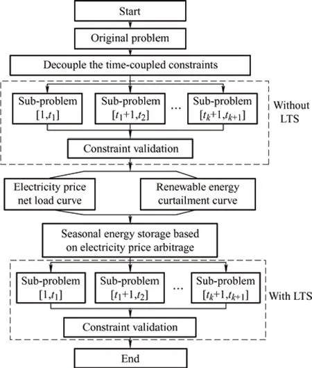
Fig.1 Long-term operation procedure with LTS

Step 1: Construct the UC model without LTS,as formulated in Eq.(31).The UC problem is divided intoKsub problems,which can be easily solved in parallel,as shown in Eq.(32).This is because the time-coupled constraints (e.g.,ramp rate and minimum on/off time constraints of the thermal units) between the different sub problems are removed.

Step 2: Construct a feasible solution for the UC model without LTS based on the solutions from all the sub problems in Step 1.The solutions between adjacent sub problems must be verified to satisfy the time-coupling constraints.Otherwise,the solutions of the sub problems must be adjusted to satisfy the temporal coupling constraints.Section 3.4 describes the validation process.

Step 3: Optimize the annual discharging/charging schedule of the LTS.The LMP,net load curve,and on/off states of the units are obtained in Step 2.As shown in Eqs.(5)-(11),the SOC targets of the LTS that can be integrated into the UC with LTS as the SOC constraints are optimized by solving the model.

Step 4: Construct a solution for the original long-term UC model with LTS,as shown in Eq.(33).The initial and end SOCs of the LTS in each sub problem are set as constraints that can decouple the original UC with LTS into independent sub problems.

3.2 UC model without LTS

The UC model without LTS is constructed based on the UC model with LTS in Eqs.(12)-(30),whose compact forms are as follows

whereC(·) denotes the variable cost function of the thermal unit,represented by the first term in Eq.(12).A1denotes the coefficient matrix for the associated constraint variables,andd1denotes the constant column vector.In Eq.(31),the first row reflects the power balance constraint and the second row represents the inequality constraint consisting of Eqs.(14)-(16) and Eqs.(18)-(25).The third row represents the binary variable constraint for the units,as expressed in Eq.(17).Eq.(31) is a mixed-integer programming problem with two time-coupling constraints: minimal on/off time and ramp rate constraints.

Horizon splitting is used to decouple the time-coupling constraints,resulting inNksub problems.The mathematical models of the sub problem can be represented as follows

wheretkis the time interval for thek-th subproblem.For instance,8 760 h in a year can be divided into 365 days,Nk=365,t1=0,t2=24,…,t365=8 760.Whenk=1,the initial state and online/offline duration of the units are assumed to be given,and the state and online/offline duration at the end of the problem are not constrained.Whenk>1,the initial and end states and the online/offline duration of the units are not constrained.Therefore,the UC model in Eq.(30) can be decoupled intoNksub problems,which can be solved in parallel.The optimal solution fork-th sub problem is

3.3 UC model with LTS

A feasible solution to Eq.(32) is obtained by solving the sub problems in parallel.Subsequently,the LMP,net load curve,and renewable energy curtailment can be obtained.The temporal profile of the SOC of the LTS is obtained by solving the price-arbitrage model in Eqs.(5)-(11).To decouple the time-coupling constraints of the LTS,the SOC targets are used for the initial and end of each sub problem in Eq.(32) as the boundary constraints.In Eq.(33),the first row reflects the balance of power in the power system,and the second row is an inequality constraint that includes Eqs.(2),(3),(14)-(16),(18)-(27),and (29).The third row is an inequality constraint that includes Eqs.(1),(4),and(28).Eq.(4) indicates that the SOC at the initial and final time intervals of each sub problem should be equal to the SOC obtained by solving the model in Eqs.(5)-(11).The fourth row is the same as in Eq.(17).

whereA2andA3denote the coefficient matrices of the corresponding constraints.d2andd3denote the constant column vectors.

3.4 Construction of a feasible solution

The constraints for all successive solutions,and,are validated,including the minimal up/down time and ramp rate constraints.Assuming that in thek-th sub problem,generatorgrequires re-dispatch periodsag,kat the end of the time interval[tk+1,tk+1] and periodsbg,kat the beginning of the time interval [tk+1+1,tk+2] in the (k+1)-th sub problem.The four cases are as follows.

Case (1)Ug,tk=1 andUg,tk+1=0: Generatorgis online at the end of the time interval [tk+1,tk+1]and offline at the beginning of the time interval[tk+1+1,tk+2].

In Eq.(34),ifPg,tk-Pg,tk+1≤andτgk≥,then the minimum uptime constraints and ramp-up limitation are satisfied.The power output of generatorgdoes not require adjustments.Ifτgk<,the minimum uptime constraints are not satisfied.The on/off status of generatorgmust be adjusted.IfPg,tk-Pg,tk+1≥,the ramp-up limitation is not satisfied,and the output of generatorgmust be adjusted.In Eq.(35),the discussion is similar to that of Eq.(34).

To illustrate the constraint validation procedure,Fig.2 shows an example of Case (1).The minimum up and down times for unitgare set to 4 h and 2 h,respectively.Unitgis started online for 2 h before the end of thek-th period and shut down for 3 h following the beginning of the (k+1)-th period.Here,τg,tk=2 and=3.When generatorgsatisfies the ramp-up rate constraints,ag,k=4 andbg,k=0; otherwise,ag,k=4 andbg,k=1.

Fig.2 Illustration of constraint validation

Case (2)Ug,tk=0 andUg,tk+1=1: This means that generatorgis offline at the end of the time interval[tk+1,tk+1] and online at the beginning of the time interval [tk+1+1,tk+2].

Case (3)Ug,tk=1 andUg,tk+1=1: Generatorgis online at the end of the time interval [tk+1,tk+1]and the beginning of the time interval [tk+1+1,tk+2].

Case (4)Ug,tk=0 andUg,tk+1=0: Generatorgis offline at the end of the time interval [tk+1,tk+1]and the beginning of the time interval [tk+1+1,tk+2].

Note that the period of violation of the constraint for the generators is different.The longest period among all the generators is selected as the period for re-dispatch.

Thus,the period that must be re-dispatched between two consecutive sub problems is [tk-ak,tk+bk],calculated using Eq.(32) with the time interval[tk-ak,tk+bk].The re-dispatch model is established using Eq.(33).

4 Case study

Numerical tests were conducted on a modified IEEE 24-bus system in which one LTS,two wind farms,and two solar farms were introduced,to validate the effectiveness of the proposed method.All simulations were run using GUROBI under YLMIP with a duality GAP of 0.1%.

4.1 Case overview

The IEEE 24-bus system comprised 16 thermal units and 38 transmission lines.The total capacity of the thermal power plants was 3 365 MW.The wind farms were connected to nodes 3 and 5 with a rated capacity of 500 MW.The solar farms were connected to nodes 7 and 13 with a rated capacity of 1 000 MW.The LTS was connected to node 13.The rated capacity of the LTS was 500 MW/84 000 MW·h with a rated discharging hour of 168 h.The charging and discharging efficiencies of the LTS were 60% and 90%,respectively.The rated capacity of the LTS accounted for approximately 16% of the renewable installed capacity,which is within a reasonable range for most Chinese provinces.The parameters regarding the load demands,generation profiles of renewable energy,and parameters of generators were obtained from Ref.[25].

The four scenarios are as follows.The UC for an 8 760 h chronological optimization problem was used to test the proposed method.The length of the time interval was 1 h and the length of the time horizon was 1 year.The duration of each period of 1 day has 24 h.Thus,the annual optimization problem can be split into 365 sub problems.S1 was used as the benchmark for comparison with the proposed method.S2 was used to test the proposed method.S3 was used to study the impact of different rated discharging hours of the LTS on the solving efficiency.S4 was used to investigate the impact of the number of sub problems on the solving efficiency.

S1: The original UC.

S2: The original UC was solved using the proposed method.The original UC was split into 365 sub problems that could be solved in parallel.

S3: The original UC was solved using the proposed method.The rated discharge hours were set to 6 h,24 h,and 168 h.

S4: The original UC was solved using the proposed method.The length of the sub problem was set to 2 days,4 days,and 7 days.The length of the time horizon was 1 month.

4.2 Effect of different solving scenarios

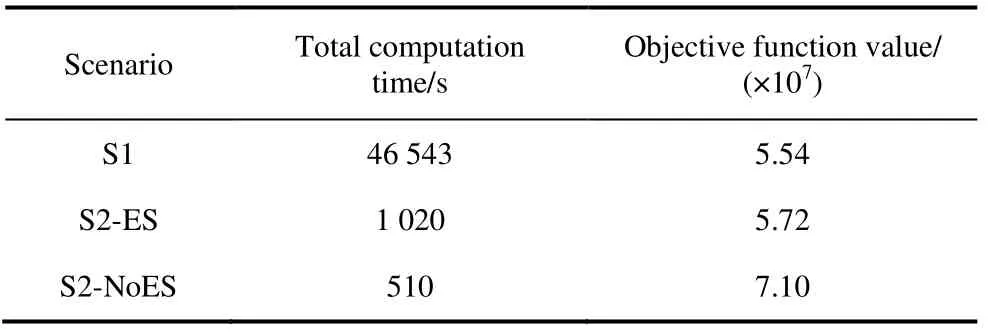
Tab.1 shows the computation times and objective function values for S1 and S2.The objective function value of the original UC problem was 5.54×107.The computation time was 46 543 s.Scenarios S2-ES and S2-NoES represent the original UC with and without LTS,respectively.The computation time in S2-ES decreased by 97.8% with a relative error of 3.3% compared with the original problem.

Tab.1 Results of different scenarios

Fig.3 shows the net load and renewable curtailment without LTS for S2-NoES.The renewable curtailment in Summer and Winter is lower than that in Spring and Autumn owing to the high load demand.Moreover,the objective function value of the system increased from 5.74×107to 7.11×107.Fig.4 shows the net load and curtailment with LTS for the S2-ES.The curtailment decreased by 75% compared with the S2-NoEs.These results indicate that the deployment of an LTS can support the integration of renewable energy by reducing curtailment.

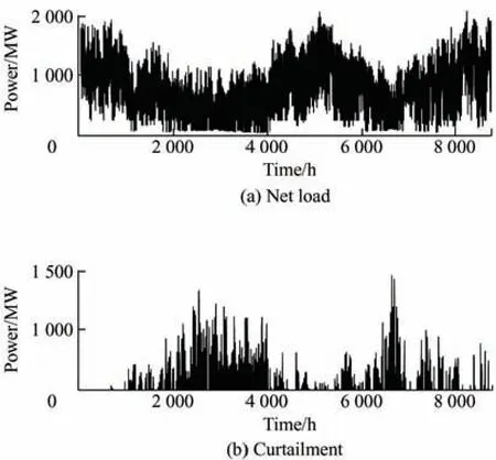
Fig.3 Net load and curtailment without LTS

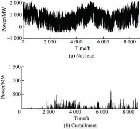
Fig.4 Net load and curtailment with LTS

The daily SOC curves for S1 and S2 are shown in Fig.5.The trend of SOC in S2 was consistent with that in S1.This discrepancy is caused by errors in the transmission load constraints or solutions to the sub problems.Nevertheless,Fig.4 indicates that the LTS optimization in S2 can reach a global optimum.The basic concept of operating an LTS is to charge renewable curtailment in spring and discharge it to supply power in summer.

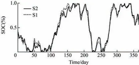
Fig.5 Daily SOC curve of LTS

Thus,for systems with a high penetration of VRE,the proposed method can not only reduce the computational burden drastically but also decrease renewable curtailment through seasonal energy shifts.

4.3 Effect of discharging hours

Tab.2 shows the results of the UC with different rated discharging hours of LTS.The total computation time for all scenarios exhibited no significant increasing trend.As the rated discharge time increased,the renewable curtailment increased slightly,whereas the value of the objective function decreased.For example,when the rated discharging time of the LTS was set to 168 h,the curtailment increased by 6.5%,and the total cost decreased by 5.1%,compared with the scenario with a rated discharging time of 6 h of LTS.The decrease in the total cost was due to the lack of consideration of the penalty cost in this research.

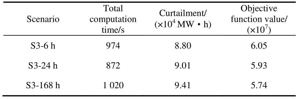
Tab.2 Results of LTS with different rated discharge times

The normalization SOC curves for different rated discharging hours of LTS are shown in Fig.6.Given the limited energy capacity,the shapes of the dispatch curves for storage durations of 6 h and 24 h had more intra-seasonal fluctuations than the corresponding dispatch curves for storage durations of 168 h.

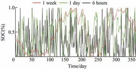
Fig.6 SOC curves of LTS for different discharge times

4.4 Effect of the number of sub problems

Tab.3 shows the results for different scenarios with different numbers of sub problems in one month.As the number of sub problems decreased,the relative error of the solution decreased.When the length of each time interval was one week,although the computation time increased from 121 s to 1 530 s,the relative error decreased from 4.6% to 1.0% compared with the scenario with a time interval of 1 day.Thus,a reasonable time interval must be selected for the sub problem to balance the trade-off between solving efficiency and errors.

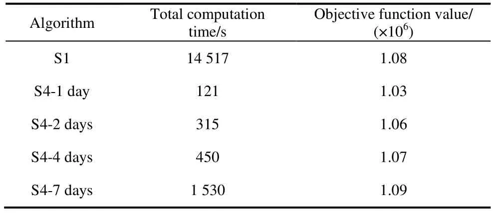
Tab.3 Results of different numbers of sub problems in one month

5 Conclusions

UC with time-coupled constraints between consecutive faces presents a significant computational burden.A bi-level optimization approach is proposed to solve long-term UC with LTS based on time-horizon splitting.The upper-level model solves the UC without LTS using a time-horizon splitting approach to perform a chronological simulation of the power system.The lower-level model solves the price-arbitrage model of the LTS to optimize its yearly operation based on LMPs.The lower-level model is used to generate the SOC targets at the end of each sub problem.The upper-level model is then run again with the SOC targets of the LTS as constraints.Thus,the UC model with the LTS can optimize the hourly operation of the LTS while following the yearly dispatch shape defined by the price-arbitrage model.Case studies using a modified IEEE-24 system showed that the computation time can be significantly reduced by 97.8% using the proposed method.