Simple and robust h-adaptive shock-capturing method for flux reconstruction framework

Linto HUANG, Zhenhu JIANG, Shui LOU, Xin ZHANG, Cho YAN,*

a School of Aeronautic Science and Engineering, Beihang University, Beijing 100191, China

b Research Office No.12, Beijing Institute of Astronautical Systems Engineering, Beijing 100076, China

KEYWORDS Adaptive mesh refinement;Flux reconstruction;Positivity-preserving scheme;Robustness;Shock-capturing

Abstract In this paper, a simple and robust shock-capturing method is developed for the Flux Reconstruction (FR) framework by combining the Adaptive Mesh Refinement (AMR) technique with the positivity-preserving property.The adaptive technique avoids the use of redundant meshes in smooth regions, while the positivity-preserving property makes the solver capable of providing numerical solutions with physical meaning.The compatibility of these two significant features relies on a novel limiter designed for mesh refinements.It ensures the positivity of solutions on all newly created cells.Therefore, the proposed method is completely positivity-preserving and thus highly robust.It performs well in solving challenging problems on highly refined meshes and allows the transition of cells at different levels to be completed within a very short distance.The performance of the proposed method is examined in various numerical experiments.When solving Euler equations, the technique of Local Artificial Diffusivity (LAD) is additionally coupled to damp oscillations.More importantly, when solving Navier-Stokes equations, the proposed method requires no auxiliaries and can provide satisfying numerical solutions directly.The implementation of the method becomes rather simple.

1.Introduction

For the purpose of having accurate and well-resolved results of fluid dynamic simulations, various numerical methods have been developed by many researchers.1–5In recent years,high-order methods6–11are widely used or studied because of their better accuracy and lower numerical dissipation.They can be applied to the simulation of complex problems, and are competitive in providing solutions within a given error.12However, some shortcomings of them prevent their further application.For example, high-order methods usually lack robustness.When faced with tough problems containing violent change in states, strong shocks, or vacuums, high-order solvers are fragile and easy to blow up.Besides, high-order methods can be very costly.When finer meshes or higherorder bases are used to improve the resolution of flow structures, total degrees-of-freedom increase quickly and the cost of the computation perhaps becomes unacceptable.

The above two facts require more consideration on the topic of shock-capturing.The discontinuous nature of shocks makes them hard to be sharply and monotonously identified.If a mesh of smaller size is used,shock solutions will be located within a narrower space, but the cost of the computation will significantly increase.In addition, strong oscillations near the shocks can produce unphysical solutions.The existence of negative densities or pressures leads to ill-posedness of the initial value problem of gasdynamic equations,13which may be fatal for high-order solvers because of their lack of robustness.

Flux Reconstruction(FR)14(or known as CPR(Correction Procedure via Reconstruction)) provides us with an ideal framework for the studies on shock-capturing.It is a Discontinuous Galerkin (DG)-type method which can recover other high-order methods like Nodal Discontinuous Galerkin(NDG)15and Staggered-Grid (SG).16,17Besides its inherent advantages shared by many DG-type methods including stencil’s compactness, geometric flexibility, and hp-adaptivity, it is also considered to be highly efficient.18,19Here, we apply the AMR technique to this efficient framework to identify shocks and refine meshes in nearby regions.h-adaptivity is chosen,because it is more preferable than p-adaptivity in discontinuous flows,20and simpler than hp-adaptivity.In this way, the rapid growth in computational cost caused by uniform refinement is avoided.The research in Refs.21,22provides a valuable reference.

Like other high-order methods, FR is not robust enough for solving strong shocks.Incorrect negative density or pressure values may arise during computations.Its improvement in robustness can be achieved by combining the property of positivity-preserving, which is a restriction in the physical aspect and is naturally satisfied by many low-order methods.The study on positivity-preserving property has attracted great attention for many years.Inspiring works23–29realize this property in high-order frameworks.Remarkable robustness enhancement is observed in their numerical tests.On this issue,one of the most successful works is seen in Refs.13,30–33.The positivity-preserving scheme proposed in these papers is suitable for general DG-type spatial discretizations, and can be applied to various equations on different types of elements.We follow this work to realize the positivity-preserving property in the FR framework.However, mesh cells may be combined or divided during h-adaptive refinement.The positivity of the solutions on these newly created cells remains uncertain.We prove that the approach of cell combination in this paper will naturally guarantee positivity, and then design a special positivity-preserving limiter for cell h-subdivision.Therefore,the proposed adaptive method is completely positivitypreserving.

In this paper, the performance of the proposed shockcapturing method is well examined.The adaptive solver shows its consistent high robustness in various numerical experiments.When solving Euler equations, we combine it with the Local Artificial Diffusivity (LAD) technique34–37to smooth oscillations.The LAD is in the same form of physical viscosity,so its influence on positivity can be referred to in Ref.13.When we solve Navier-Stokes equations under a given Reynolds number, no other techniques are needed.Satisfying results are provided by the solver as well, which means that the proposed method is able to provide nonoscillatory shock solutions in high local resolution directly.

The rest of this paper is organized as follows.The twodimensional governing equations and the FR discretization are introduced in Section 2.The technical details of the adaptive method are shown in Section 3.In Section 4, we discuss how to realize the positivity-preserving property.Then,in Section 5, we evaluate the performance of the proposed method by one- and two-dimensional experiments.Finally, in Section 6, the conclusions about the proposed method are given.

2.Governing equations and spatial discretization

2.1.Governing equations

We focus on two-dimensional equations in the conservative form:

where μ is the shear viscosity given by the Sutherland formula;38β is the bulk viscosity, and it is equal to 0 according to the Stokes hypothesis; is the unit tensor.

2.2.FR discretization

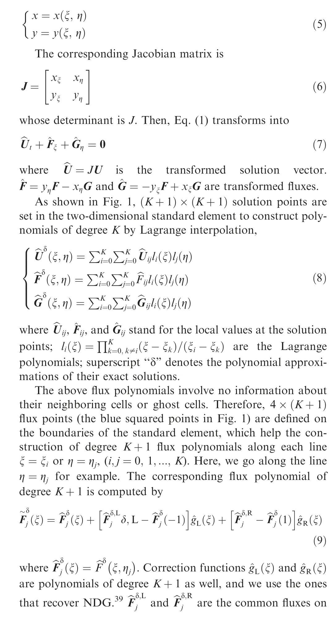
Suppose there is a coordinate transformation from the twodimensional standard element [-1,1]× [-1,1] (see Fig.1) to an arbitrary quadrilateral element,

Fig.1 Solution points(black dots)and flux points(blue squares)in two-dimensional standard element (K = 2 for example).

3.Algorithms for mesh refinement

3.1.Data management

The choice of data management strategies40–42is critical in the application of the Adaptive Mesh Refinement (AMR) technique.The resulting methods may have distinct performance in memory requirement,43–45computational cost, or efficiency(parallel or not).However, the proposed adaptive shockcapturing method is independent of the data management strategies that we choose.In the present work,we only suppose that correct information about cell neighbors is offered, and do not focus on the comparison between adaptive refinements and uniform refinements temporarily.

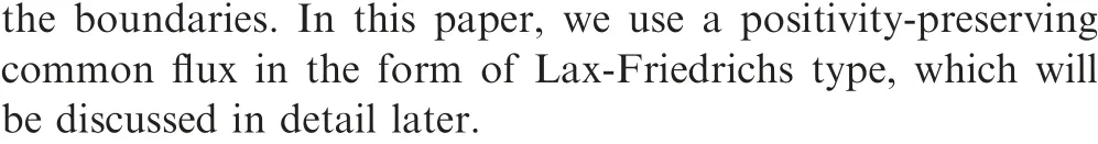
We use a data management strategy21,46in which the information on each cell is directly retrieved.In the program, a unique label number is assigned to each cell.This label number not only distinguishes cells, but also interprets their hierarchical relationship.For example, when a quadrilateral cell with the label number l is divided,the label numbers of its four children cells Li(i=0,1,2,3) are

where N is the total number of level-0 cells in the beginning.This incremental relationship bridges cells at different levels in a simple way.When cells are divided, the label numbers of the newly created cells are computed by that of their parent cell.And when these cells are recombined, the inverse of Eq.(11) determines the unique label number of the parent.Fig.2 illustrates this regulation.

A contiguous memory management strategy is also adopted to improve the compactness of storage.We recommend Ref.21for the details.

3.2.Refinement criteria

This subsection introduces the criteria for mesh refinement.First of all, a critical principle is stressed by many h-adaptive methods, i.e., cells that share a common edge should have differences in levels not greater than one.This principle involves an important assumption called proper-nesting.

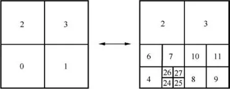
Fig.2 An example of label numbers (N = 4 for example).The order of the level-0 cells is arbitrary.

As shown in Fig.3, owing to the principle, high-level cells are surrounded by low-level ones, and non-conforming interfaces are all restricted to 1–2 configuration.It reduces the complexity of algorithms greatly.

Then,we shall discuss which cells are combined or divided.The parameter Ir reflects the necessity of refinement of each cell.It may be values based on error or adjoint solution47–50.When a boundary layer is involved, the parameter can be the velocity derivative uy.In this paper, we focus on the capture of shocks, so we choose Ir=f (∇∙u）, where f(∙）is a function related to the velocity divergence.The gradient of density ∇ρ is additionally considered for cases including nonnegligible contact discontinuities.

Based on Ir, the below two criteria of refinement can be followed:

(1) Fixed number or percentage of cells are combined or divided.We regard their Ir as smaller than a lower cut-off value Irlowor greater than an upper cut-off value Irupp.Then, a cell with label i is combined if

Here,we suppose cell i is the first one of four children cells created by a previous division.This combination cannot violate the proper-nesting assumption as well.On the other hand,cell i is divided if

where clowand cuppare adjustable coefficients with suggested values in 0.1–0.4 and 1.0–1.5.

3.3.Damping oscillations

The LAD36is added to suppress oscillations when we solve the compressible Euler equations.It is in the same form of physical viscosity.The coefficients of artificial shear viscosity μ*, bulk viscosity β*, and thermal conductivity κ*are

where Cμ, Cβ, and Cκare user-specified constants; S, ∇∙u,and e are the magnitude of the strain rate tensor, the dilatation, and the internal energy, respectively; ξlrepresents the computational coordinates ξ and η;xmrepresents the physical coordinates x and y;⊿lstands for the physical mesh spacing in ξldirection; ρ,c, and T are density, sound speed, and temperature,respectively;the overbar denotes an appropriate smooth function.The restriction-prolongation filter introduced in Ref.36is recommended.

In this paper, we use the following simplified version:

where a switching function fβ=H(-∇∙u）is added to blank expansion and H is the Heaviside function.

Remark 1.In the previous subsection, Ir=f(∇∙u）is introduced to quantify the necessity of refinement.When we solve the Euler equations with the LAD terms, since β*needs to be computed and is large in shock cells,it will be convenient to set Ir=β*, i.e., directly using β*to indicate the mesh refinements near shocks.Extra computational costs are thus avoided.When solving Navier-Stokes equations,only the single parameter Ir=β*is still computed to indicate mesh refinements as usual.No artificial viscosity terms are added.In this case,other indicators such as those in Ref.52can be applied instead.

Fig.3 Examples of mesh refinement under proper-nesting assumption.Cells marked by triangles are divided.

3.4.Projection method

To maintain the conservation of the shock-capturing method,the L2projection53is used to evaluate the solutions on all newly created cells.As shown in Fig.4, if we write all the values at the (K+1）× (K+1）solution points in column vectors,i.e., Q for the parent cell on the left and qi, qi+1,qi+2, qi+3for the children cells on the right, the results of L2projections satisfy

Specially, h-subdivisions do not change the degree of solution polynomials.Therefore,we can simply divide the solution polynomial on the parent cell U(x ）into four parts(see Fig.5).The results of Eq.(18) should be consistent with these four parts, respectively.This property is useful for the design of the positivity-preserving limiter in Section 4.3.

The mortar method is adopted to compute common fluxes(see Section 2.2) when 1–2 interfaces arise.It maintains global conservation as well.We recommend Ref.17for reference.

4.Realization of positivity-preserving property

4.1.Definition of positivity

The high robustness of the proposed shock-capturing method relies on the realization of the positivity-preserving property.Denoting the solution vector as U, we hope that it belongs to the following admissible set:13

so its density,pressure,temperature,and internal energy are all positive.ε is a small number (10-13) to replace 0.

The above positivity ensures the physical meaning of numerical solutions, and also relates to discrete L1stability.28However, the positivity of solutions may not hold in many high-order schemes including FR.When the AMR techniques are applied, how to preserve the positivity of solutions on newly created cells also remains to be considered.We will discuss these two aspects in the next subsections.

4.2.Implementation of positivity-preserving FR scheme

The proposed adaptive shock-capturing method in the FR framework keeps the positivity of solutions at any explicit time.Without regard for mesh refinements temporarily, the positivity-preserving property can be realized by the following steps:

Step 1.The initial condition gives the field at t=t0, in which the average solution on each cell is positive.

Step 2.At t=tn(n=0,1,2...), if the average solution on each cell is positive, we enforce the positivity of the solutions at a set of quadrature points that we choose (see Remark 3 and Fig.6) by scaling each solution polynomial U (x ）around its average.The following high-order accurate limiter is used:

(1) Scaling density ρ

Fig.4 An example of cell combination and division.Solution points (black dots) are also shown (K = 2 for example).

Fig.5 An illustration of L2 projection from parent cell to child cell i.

Fig.6 An example of quadrature points in standard element.Solution points(black dots)and flux points(blue squares)are also shown on the left(K=2 for example).The solution points of FR are the 3×3 Legendre-Gauss points.The flux points are at the boundaries.The quadrature points that we choose are marked by crosses on the right,which are obtained by the tensor product of three Legendre-Gauss points and three Legendre-Gauss-Lobatto points in x and y directions.

where L(U ）stands for the residual of a current solution U.The maximal time step Δt meets a Courant-Friedrichs-Lewylike limit proportional to the mesh spacing:

where ω is a constant related to the choice of the quadrature points.It is worth noting that the positivity at each inner stage should also be enforced.

The solution at t=tn+1is proven to have positive cell averages after the last step.13Consequently,by repeating Step 2 to Step 4, the positivity of solutions at any given time is guaranteed.

Remark 2.In the above steps, two important restrictions are involved to ensure the positivity of cell averages.One is for α.Eq.(24) indicates that it should be large enough.We suggest the use of local Lax-Friedrichs flux in practice, that is α=ρ(A ）, where ρ(A ）is the spectral radius of matrix A=∂F/∂U.It usually satisfies the restriction and avoids the evaluation of Eq.(24).The other restriction is for Δt.Eq.(26)is only a sufficient condition for the preservation of positivity.In practice, we still determine it by the stability requirement,and use a half Δt if the positivity fails.Eq.(26) ensures that it will end after finite loops.

Remark 3.The quadrature points that we choose should satisfy:(A)They can evaluate the integral of the solution polynomial exactly.13,32(B) The flux points of the FR discretization are covered.For example, on the left of Fig.6, the solution points of FR are the 3×3 Legendre-Gauss points.The corresponding flux points are also displayed.Then, the quadrature points can be the cross-marked points on the right.This is a convenient choice because the quadrature points coincide most with the solution points and the flux points, where the local solutions are already known.In Ref.13, an efficient implementation is also introduced.

4.3.New positivity-preserving limiter for AMR methods

In the previous subsection, the solution at t=tn+1has positive cell averages after the last step (i.e., Step 4).Before we go to Step 2 and repeat the cycle, the cells in the mesh may be combined and divided with the motion of shocks.We ought to ensure the positivity of the average solutions on these newly created cells, so that Step 2 of the new cycle can continue.

The following theorem clarifies the natural positivitypreserving property of cell combinations:

Theorem 1.The average solution on a newly created parent cell is positive, if the average solutions on its children cells are all positive and the L2projection is used to evaluate this new solution.

Proof of Theorem 1.Because the L2projection(see Section 3.4)is used, the new solution on the parent cell U(x ）satisfies

On the other hand,if a parent cell is h-subdivided,the average solutions on all newly created children cells (evaluated by L2projection)may not be positive,since the inverse of Eq.(30)is not always true.The creation of children cells with negative average solutions is indeed observed in the program.

In this paper, we introduce a new limiter for h-subdivision to ensure the positivity on all children cells.This limiter works before a cell is h-subdivided.It adjusts the solution on this cell in advance.Then, the L2projection can proceed as usual to evaluate the solutions on the newly created children cells.The results of projection will be naturally positive.

Fig.7 illustrates a cell which is to be divided.We denote the solution polynomial on this cell as U(x ）.In Fig.7, the crossmarked points are in fact the previously chosen quadrature points of the child cell i (see Fig.6).Other quadrature points of cell i+1 to cell i+3 are not displayed for clarity.

Before the h-subdivision, we adjust U(x ）by the same scaling equations (Eq.(21) and Eq.(22)) to enforce the positivity at the cross-marked points.Then,after the division and the L2projection, the solutions at the cross-marked quadrature points of child cell i will all be positive.Meanwhile,the average solution on cell i is positive.Because the corresponding quadrature law is exact for the cell average, i.e.,

Therefore, the average solution on child cell i is positive.The cases for the remaining children cells i+1 to i+3 are similar.

The performance of the new positivity-preserving limiter for h-subdivision can be concluded from the following aspects:

(1) Simplicity.The new limiter uses the same scaling equations Eq.(21) and Eq.(22) as the limiter in Section 4.2,except that the solutions at different locations are adjusted.We can use the same structure of programs,so its realization is simple.

Fig.7 Locations where the solutions need to be adjusted by new limiter for h-subdivision.Only those in the first child cell are shown(marked by crosses).The quadrature points in each subcell are the same as those in Fig.6.

(2) Accuracy.Both the limiter in Section 4.2 and the new limiter adjust solution polynomials by scaling.In Ref.13, the high-order accuracy of this type is demonstrated.

(3) Conservation.This type of scaling limiters do not change cell averages, so they are conservative.Together with the conservation in the FR discretization, the evaluation of common fluxes, and the L2projection, global conservation of the proposed shock-capturing method is guaranteed.

(4) Economy.Owing to the limiter, the solutions at the quadrature points of the children cells are naturally positive after L2projections.They need not be adjusted again at the beginning of the new cycle (i.e., Step 2 in Section 4.2).The new limiter for h-subdivision actually completes the scaling of the solution polynomial in advance on the parent cell and requires no extra cost.

The compatibility of the positivity-preserving property and the AMR technique relies on this new limiter for h-subdivision.In the numerical tests, the proposed method shows high robustness even when using high-level refined meshes to solve tough problems.The transition of different cell levels is allowed to be completed in a very short distance.

For other problems such as equations with source terms,55gaseous detonations,56,57and multi-phase flows,58their definitions of positivity and the scaling expressions are more or less different.However, the proposed limiter for h-subdivision is applicable to all these problems.

5.Numerical results

In this section, the performance of the proposed shockcapturing method is examined in numerical experiments.When solving one-dimensional problems, Euler equations coupled with the LAD and Navier-Stokes equations are both involved.In two-dimensional problems, we focus on Navier-Stokes equations, and the shock solutions on high-level refined meshes are obtained under the restriction of positivity only.

5.1.Convergence study

We use a similar test in Ref.32to demonstrate the convergence of the proposed AMR method in the FR framework.In the periodic domain [0, 2π], we give the following smooth initial condition:

The minimum density is 10-2.Since no shocks exist in this smooth test, we refine meshes in low density regions.A constant rate of refinement r=0.3 is set, i.e., thirty percent of low-level cells are refined to next levels.The positivity limiters get turned on in this test.

In Table 1 and Table 2, the L1and L2norm errors are reported, respectively, to check whether the expected orders of accuracy are achieved.Two mesh levels are set in this case.It is shown that the adaptive FR discretization using PKbasis(from P1to P3)maintains correct (K+1）-th order of accuracy.

Then, in Table 3, we focus on the L2errors of the FR discretization using P2basis only.Two mesh levels are used still.This time, the rate of refinement increases from r=0.3 to r=0.7, which means that more high-level cells are set in the domain.We can see that the L2norm errors reduce rapidly with this increase, and the accuracy of the adaptive discretization maintains the third order.

Finally, in Table 4, we change the total numbers of mesh levels.The L2errors of the adaptive FR discretization using P2basis are shown.The refinement rate r=0.3.It is observed that the L2errors also reduce when more mesh levels are set,and the accuracy is the third order.(Here, the level-1 refinement represents that only the uniform basic cells are used.)Besides, the errors of the level-2 and level-3 refinements are close, because the errors from the low-level cells dominate in this case.

5.2.Sod problem

Consider a mild Riemann problem with the initial condition,

The terminal time is 0.25.This solution contains a rarefaction, a contact discontinuity, and a shock.

Navier-Stokes equations are solved first.We choose an appropriate Reynolds number Re=10000 to reflect the effect of adaptive refinement.In Fig.8,the density values at all three solution points in each cell are displayed.The zoomed figure ison the right, in which the locations of the cell borders are marked in the top.When the number of uniform cells N=100, 200, the solutions are oscillatory near the shock.However, the density solution on 100 basic cells with level-4 refinement is sharp and nearly monotone.This confirms the phenomenon reported in Ref.13that we can get satisfying shock results on fine meshes under the restriction of positivity only.

Table 1 L1 norm errors of adaptive FR method using different bases.

Table 2 L2 norm errors of adaptive FR method using different bases.

Table 3 L2 norm errors of adaptive FR method using different rates of refinement.

Table 4 L2 norm errors of adaptive FR method using different refinement levels.

In Fig.9, artificial viscosity is added to the compressible Euler equations.This artificial viscosity not only indicates the location of shock but also smooths the solution.When using the same coefficients of Cμand Cβ, the shock solution on the adaptive mesh is steeper than those on the uniform meshes,because the amount of the artificial viscosity is related to the mesh spacing.The contact discontinuity in the middle is less affected by the simplified LAD that we use.

5.3.Lax problem

This is a challenging Riemann problem with the initial condition59:

The computation is finished at t = 1.3.

Without the restriction of positivity-preserving, the original FR method is easy to fail in this test.We first solve Navier-Stokes equations under Re=1000.Fig.10 illustrates the pressure results on different meshes.The oscillations on the adaptive mesh almost disappear compared with those on the uniform meshes.Then, the compressible Euler equations coupled with the LAD are solved.As shown in Fig.11, the artificial viscosity term correctly indicates the location of the shock and triggers local level-4 refinement.The thickness of the shock on the adaptive mesh is much thinner.

5.4.Shock collision problem

This tough problem in Ref.38which is made up of the left and right shocks in the blast wave problem of Woodward and Colella60mimics the collision of two strong shocks.The initial condition is

Fig.8 Density results of Sod problem.Navier-Stokes equations under Re = 10000 are solved.

Fig.9 Density results of Sod problem.Euler equations with LAD are solved.The coefficients of LAD are Cμ = 0.2 and Cβ = 2.0.

Fig.10 Pressure results of Lax problem.Navier-Stokes equations under Re = 1000 are solved.

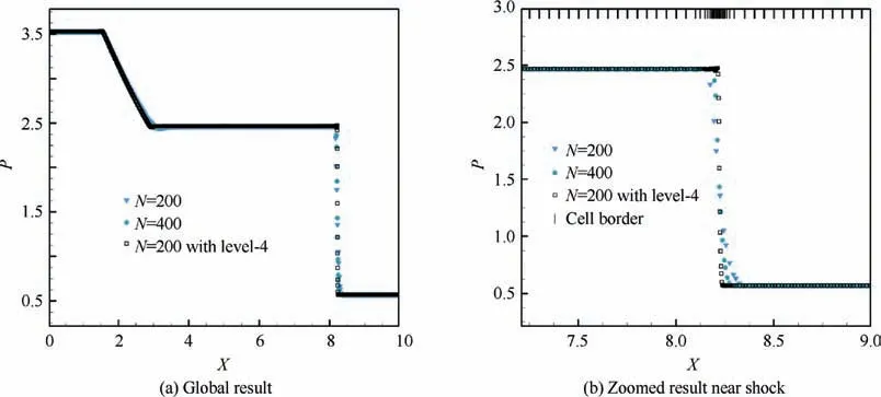
Fig.11 Pressure results of Lax problem.Euler equations with LAD are solved.The coefficients of LAD are Cμ = 0 and Cβ = 2.0.

The end time of this test is 0.035.

Fig.12 illustrates the density results of Navier-Stokes equations under Re=2000.The zoomed figure is also included.The solutions on the coarse equidistant meshes have violent oscillations near the locations of shocks.However, when the level-6 adaptive mesh is used, the shock solutions are sharp and less oscillatory.More importantly, the change of mesh spacing with the maximal ratio of 32 is completed in a very short distance (about 0.01), which reflects the high robustness of the proposed method.

In Fig.13, we turn to show the pressure results of Euler equations.The details of the shock on the right are also displayed.The coefficients of the LAD are Cμ= 0 and Cβ= 2.0.It can be seen that we obtain a steeper solution by using level-4 mesh refinement.

5.5.Sedov blast waves

This is a point-blast wave test which includes low pressures and strong shocks.51In the region [0,1.1]× [0,1.1], we set the following initial condition:

where Δx=Δy=1.1/40 is the spacing of the basic mesh.As for boundary conditions, the left and bottom boundaries are symmetric.Outflow conditions are applied to the rest.We take ε=10-13in Eq.(21) and Eq.(22) and stop the computation when t = 0.001.

In fact, we consider a quarter of the whole domain in this test.A very large value of pressure is assigned to the cell closest to the origin, so the physical meaning of this test may be limited.However, it provides another important evidence of the robustness of the proposed shock-capturing method.

Fig.14 illustrates the pressure solution of Navier-Stokes equations under Re=100000.Cells in five levels are set in the mesh.On the left, the contour is displayed.On the right,the detailed distribution of pressure along the diagonal x-y=0 is shown.The shock solution is sharp and thin, and better than that on the 160×160 uniform mesh.No apparent oscillation occurs near the discontinuity in the curve.

Fig.12 Density results of shock collision problem.Navier-Stokes under Re = 2000 are solved.

Fig.13 Pressure results of shock collision problem.Euler equations with LAD are solved.The coefficients of LAD are Cμ = 0 and Cβ = 2.0.

Fig.15 compares the contours of β*on the level-3 and level-5 refined meshes.This coefficient of bulk viscosity only works as the refinement indicator here.In each figure, the choice of Cβis not important,since we divide or combine cells according to their relative values.The thickness of the shock is greatly reduced when the higher-level refinement is applied.

Fig.16 compares the meshes using level-3 and level-5 refinement.Owing to the h-adaptive technique,the shocks are solved on 1/4 and 1/16 smaller cells compared with the basic ones.

5.6.Double Mach reflection

The classical double Mach reflection problem is solved to further test the performance of the proposed method.The initial conditions and boundary conditions can be seen in Ref.61.In the domain [0,4]× [0,1], a Mach 10 shock which makes a sixty-degree angle with the x-direction meets the horizon wall.Twice Mach reflections have happened at t = 0.25 and produce two contact discontinuities.The Reynolds number is 15000.

Because of the contact discontinuities, an extra refinement indicator ｜∇ρ｜｜Ω｜3/4related to the density gradient51is additionally considered to capture them, where ｜∇ρ｜is the magnitude of the density gradient and ｜Ω｜stands for the cell volume.

Fig.17 and Fig.18 illustrate the density results on the mesh with level-4 refinement.96×24 basic cells are used.The solution displayed in Fig.17 is smooth and less oscillatory.In Fig.18,the shock structures are clear.The contact discontinuities are less dissipative owing to local refinement.

The distribution of the new indicating variable ｜∇ρ｜｜Ω｜3/4(termed as ‘‘density gradient”) is displayed in Fig.19.This new indicator triggers mesh refinement correctly at the locations of the contact discontinuities (see Fig.20) and improves their local resolution.

Fig.14 Pressure results of Sedov blast waves.Navier-Stokes equations under Re=100000 are solved.The contour illustrates pressures from 2000 to 150000 and is filled with 40 colors.The curve goes along the diagonal x-y=0.Enough points are extracted to form the curve, but we only display them at a fixed distance.

Fig.15 Contours of β* in Sedov blast waves problem.The left-contour is filled with 50 colors and displays the values from 0.5 to 7.0.The right-contour is filled with 50 colors and displays the values from 0.5 to 2.5.

Fig.16 Meshes of Sedov blast waves.The refined meshes at the terminal time are shown.

5.7.Viscous shock tube

This test shows the ability of the solver in simulating problems including viscous boundaries.A shock wave is initially located at x=0.5 and divides the computational domain[0,1]× [0,0.5] into two parts with the following states:62

Fig.17 Contour of density of double Mach reflection problem.Navier-Stokes equations under Re = 15000 are solved.This contour is filled with 24 colors and displays the values from 3 to 20.

The top wall is a symmetric boundary and the remaining walls are all non-slipping.We set 150×75 basic cells in the domain and solve the Navier-Stokes equations under a typical Reynolds number Re=200.The change of μ is omitted in this test.The end time is t = 1.0.

The indicator for contact discontinuities is also active in this test.Fig.21 and Fig.22 illustrate the density results.Complex structures caused by shock wave-boundary layer interactions such as the λ-shape shock, the separated bubble, the downstream primary vortex,and the unstable slip line are well captured by the proposed method.High-level cells are automatically set at places near these structures (see Fig.23), and thus the local dissipation is greatly reduced.

The height of the primary vortex is a significant measure of the simulation.In our computation, the height is about 0.167,which is very close to the high-order reference value 0.168 on dense meshes.63,64The density distribution along the bottom wall63,64also fits well (see Fig.24).

Besides, the magnitude of velocity derivative ｜uy｜can be used to indicate boundary layers.A Mach 0.15 flat plate problem is solved under Re=1000 for example.The boundary conditions can be seen in Ref.7.In Fig.25, representative results are illustrated.It is seen that the resolution of the boundary layer is greatly improved owing to the refinements triggered by ｜uy｜.

Fig.18 Isogram of density of double Mach reflection problem.Navier-Stokes equations under Re = 15000 are solved.24 equal spaced lines are drawn in this figure which represent the values from 3 to 20.

Fig.19 Contour of density gradient of double Mach reflection problem.This contour is filled with 30 colors and displays the values from 0.05 to 0.5.

Fig.20 Mesh of double Mach reflection problem.96×24 basic cells are set in the mesh.Level-4 refinement is applied.

Fig.21 Contour of density of viscous shock tube problem.Navier-Stokes equations under Re=200 are solved.The contour is filled with 31 colors and displays the values from 30 to 100.

5.8.Shock diffraction

In this test, a Mach 5.09 shock passes a backward facing step and diffracts at the location behind it.61The step is 1 unit wide and 6 units high,and the surfaces of it are all reflective.We use a basic mesh with size Δx=Δy=1/4 in this test and solve the Navier-Stokes equations under Re = 3000 until t = 2.3.

Fig.22 Isogram of density of viscous shock tube problem.Navier-Stokes equations under Re = 200 are solved.25 equal spaced lines are drawn in this figure which represent the values from 30 to 100.

Fig.23 Mesh of viscous shock tube problem.150×75 basic cells are set in the mesh.Level-3 refinement is applied.

In Fig.26,we show the density contours on the level-3 and level-5 refined meshes.Both contours display the values from 0.4 to 7.0.The proposed method successfully captures the inner shock and the outer shock at the same time.The shocks in the right-figure are much thinner and clearer.

Then, the isogram of density on the level-5 refined mesh is shown in Fig.27.The shocks in this figure are less oscillatory and have small thicknesses.The contour of refinement indicator β*on the same mesh is shown in Fig.28.We display the values of the highest-level cells for clarity.

In Fig.29,we focus on the development of the mesh.Four moments are recorded.It is demonstrated that the shock indicator traces the motions of the shocks well and keeps the shocks being solved on the smallest cells.

Fig.24 Density distribution along the bottom wall of viscous shock tube problem.The solid line indicates the reference value.63,64 The squares are extracted from the density contour.

Fig.25 Results of flat plate problem.

Fig.26 Density results of shock diffraction problem.Navier-Stokes equations under Re=3000 are solved.Both contours illustrate the values from 0.4 to 7.0 and are filled with 30 colors.

Fig.27 Isogram of density on level-5 refined mesh.30 equal spaced lines are drawn,which represent the values from 0.4 to 7.0.

Fig.29 Meshes of shock diffraction problem.Four different moments are illustrated.Level-5 refinement is applied.

6.Conclusions

(1) We develop a simple and robust shock-capturing method for the FR framework in this paper.This method, which combines the technique of AMR with the property of positivity-preserving, has the ability to provide smooth and satisfying gasdynamic solutions with sharp and less oscillatory shocks.

(2) The property of positivity-preserving is a significant feature of the proposed method.The realization of this property ensures the physical meaning of the numerical solutions, and enables the high-order solvers to deal with tough problems including strong shocks,low densities, low pressures, and so on.Keeping the positivity of the solutions during mesh refinement is a challenge for the method,so we prove that the positivity can be maintained if the L2projection is adopted in cell combinations, and design a limiter for cell divisions to make newly created cells all have positive solutions.The limiter can also be applied to other complex problems.

(3) The application of the LAD is an important issue in the proposed method.The LAD term smooths the numerical oscillations when we solve Euler equations,and indicates mesh refinements when solving Euler equations or Navier-Stokes equations.In the latter case, no artificial viscosity is actually added, so the numerical solutions reflect the influence of Reynolds numbers and are closer to the physical ones.

(4) The performance of the proposed shock-capturing method is well examined in one and two-dimensional tests.The shock solutions of Euler equations coupled with the LAD are sharp and thin.For Navier-Stokes equations under a given Reynolds number, nearly monotone shock results on high-level cells are also provided by the solver.These solutions do not need to be further adjusted by other techniques such as TVB (total variation bounded)or WENO(weighted essentially nonoscillatory) limiters, and thus the proposed method is rather friendly to apply.

Declaration of Competing Interest

The authors declare that they have no known competing financial interests or personal relationships that could have appeared to influence the work reported in this paper.

Acknowledgement

This research was supported by the National Natural Science Foundation of China (No.11721202).