Design and dynamic analysis of a scissors hoop-rib truss deployable antenna mechanism
2023-07-04BoHnXingkunLiJinSunYundouXuJintoYoYongshengZho
Bo Hn , Xingkun Li , Jin Sun , Yundou Xu , Jinto Yo , Yongsheng Zho ,*
a Parallel Robot andMechatronic System Laboratoryof HebeiProvince,Yanshan University,Qinhuangdao,066004,China
b KeyLaboratory ofAdvanced Forging& StampingTechnologyand Science,Ministryof Education ofChina,Yanshan University, Qinhuangdao, 066004,China
Keywords:Scissors mechanism Deployable antenna Screw theory Kinematic analysis Dynamic analysis
ABSTRACT
1. Introduction
Artificial satellites officially became a high-end equipment around the middle of the 20 centuries,with the Soviet Union 6 for launch of Sputnik 1. Fast forward to now, there are thousands of artificial satellites up orbiting earth. From the perspective of national defence security,the satellite navigation system provides the country with three independent functional guarantees of navigation,positioning and communication[1—4].As an important part of artificial satellite, deployable antenna mechanism mainly include planar antenna mechanisms, rib antenna mechanisms, ring truss antenna mechanisms,membrane antennas mechanisms,and solid surface antennas mechanisms [5—9].
In defence technology, in order to make the electromagnetic wave of radar reconnaissance satellite have lower frequency and longer wavelength,and to make the artificial satellite have a larger service range, the aperture of the deployable antenna mechanism needs to be larger. Jia [10] attempted to improve the synthesis method of metamorphic mechanisms, enabling the synthesis of parallel mechanisms. Wang [11] proposed a petal-inspired space deployable-foldable mechanism for space applications combining features common to both the flower blooming process and deployable-foldable mechanisms.Based on screw theory,Yang and Shi [12,13] synthesized rectangular pyramidal overconstrained deployable units and linear foldable over-constrained deployable unit, respectively. Han, Dai and Meng [14—16] synthesized deployable mechanisms for ring truss antennas, respectively. Liu[17] proposed a new configuration that can realize twodimensional (2D) planar deployment and designed a novel largescale 2D deployable planar antenna mechanism. Intended for large mesh antennas, Sun [18] introduced a novel deployable antenna comprising a double-ring deployable truss and a cable net reflector.Li[19]proposed a double-level guyed membrane antenna to improve the stiffness of a large-scale tri-prism deployable mast using a collapsible tubular mast. In Ref. [20], a parametric design approach to the petal-type solid surface deployable reflector was presented. Wu [21] proposed the concept of a single-layer deployable truss structure driven by elastic components, which can be applicable to small satellites,and from its stowed state,the structure is self-deployable to a planar regular hexagon configuration. All the above studies have developed typical deployable antenna mechanisms, however, their stiffness will inevitably reduce when it comes to the formation of large aperture deployable antennas,which will also reduce the accuracy of the reflective cable mesh.
Whether the deployable antenna mechanism can be successfully deployed determines the success or failure of the artificial satellite launch mission. To ensure that the deployable antenna mechanism will be successfully deployed in orbit,it is necessary to analyze the kinematic characteristics of the antenna mechanism.In Ref. [22], a method based on the equivalent concept of first removing a link and then restoring it was proposed for the DOF analysis of multiloop coupled deployable tetrahedral mechanisms.In Ref. [23], based on the aspects of flexibility and controllability through modularity and simple actuation requirements, a kinematic approach applied to a lightweight linkage structure was presented. Wei [24] studied geometry and kinematic of a planarspherical overconstrained mechanisms via closed-form equations.In Refs.[25,26],the possibility of actively controlling the stiffness of tensegrity plate-like structures throughout the changes in the selfstress level and the support conditions were explored. In another study, a general dynamic method for the deployment analysis of cable networks was proposed [27]. In Ref. [28], a large-scale deployable ring truss was introduced, which is equipped with a complete rope-driven driving method and supplements a cable net system to form a complete space antenna. Shi [29] studied the optimization of the antenna mechanism synthesis and obtained the antenna configuration with optimal stiffness and mass synthesis with a genetic algorithm. Nevertheless, the above antenna mechanisms have more than one DOFs,which will lead to a consequence of excessive using of synchronous joints,it means that the weight of the deployable antenna mechanism will become larger, and the deployment reliability of the mechanism will be reduced as the extreme temperature conditions in space may cause synchronous joints to stick.
Artificial satellites provide three functional guarantees for navigation, positioning and communication. To achieve the above functions, the dynamic characteristics of antenna mechanisms during the deployment process are also of particular importance.Wu and Zhang [30,31] proposed a dynamic method for constructing an origami dynamic model.In Refs.[32—35],a dynamic models of frame structures with clearance joints were developed.Refs. [36,37] investigated the frequency characteristics of deployable mechanisms under thermal load and in the case where the antenna was extended and locked. Siqueira [38] developed a flexible actuator finite element model which can be applied for the modeling of spatial mechanisms existing in several industrial applications. You [39] studied the deployment dynamic of a space telescope via absolute node coordinate method. Zhang [40] introduced a simplified method, which can reduce the threedimensional (3D) cell structure of the ring truss into a 2D “flattened”one.Zhao[41]presented a novel computational method for the in-situ finite element modeling of inflatable membrane structures. Their method is based on geometrical shape measurements using photogrammetry and can be used for further structural analysis.
The basic scissors mechanism unit is a planar 5R mechanism,which is symmetrical about the center of the rotational joint and has only one DOF,and it has a wide range of applications in security defence field [42—45]. A generic structure for a planar remote center-of-motion (RCM) mechanism with dual scissors-like mechanisms has been presented in Ref.[46].A centralized-driven flexible continuous robot based on a multiple scissors unit mechanism has been proposed in Ref. [47]. In that study, the kinematic and dynamic of the robot were analyzed, and its workspace and deformation performance were verified experimentally.
As introduced above,when the aperture of deployable antenna mechanism increases, the structural stiffness will decrease, which will reduce the accuracy of the reflective cable mesh. Besides, the antenna mechanism with more than one DOF will greatly increase the weight due to the excessive using of synchronous joints, and will decrease the deployment reliability of the mechanism as the extreme temperature conditions in space may cause synchronous joints to stick.In order to solve the two problems,in this paper,the position of the intermediate rotational joint of the basic scissors mechanism is changed to form an ULSM,and the original parabolic rib is replaced by the ULSM, all the ULSM s are connected to each other so that the aperture of the antenna can be constructed larger.Moreover, in order to improve the structural stiffness of the deployable antenna mechanism,the upper and lower layers of the antenna mechanism are connected by a 3R planar mechanism,the antenna mechanism forms multiple closed-loop mechanisms, so that the SHRTDAM can be obtained. When the two rods of the 3R planar mechanism are collinear, the antenna mechanism is in its fully deployed state,and the boundary singular configuration of the 3R planar mechanism prevents the antenna mechanism from deploying further.As the mechanism has only one DOF,there is no need for the synchronous joints, which can also ensure the deployment reliability. And the reflective cable mesh can be arranged at the both ends of each scissors rod,so that the SHRTDAM proposed in this paper also has the better reflective accuracy of the cable mesh.
The remainder of this paper is organized as follows.In Section 2,the SHRTDAM is proposed and its configuration and geometric characteristics are analyzed, and the DOF of the SHRTDAM is calculated in Section 3,the result showed that the mechanism has only one DOF. In Sections 4 and 5, the kinematic and dynamic models of the SHRTDAM are established based on screw theory and Lagrange equation. In Section 6, the kinematic and dynamic characteristics are calculated and simulated through MATLAB and Adams software,a ground experiment prototype of 1.5-m diameter was designed and fabricated and a deployment test is conducted,which demonstrated the mobility and deployment performance of the whole mechanism.Finally,conclusions are presented in Section 7, wherein the present work is summarized.
2. SHRTDAM configuration and geometric characteristics analysis
As illustrated in Fig. 1, the SHRTDAM consists of scissors mechanisms, nodes, and 3R planar mechanisms. The latter constitute the outer ring truss of the antenna and each rib is composed of three sets of scissors mechanisms, which connects the inner and outer nodes, each type of scissors has the same length.
To facilitate the description of the SHRTDAM,a unit mechanism is isolated to explain the characteristics of each component. The scissors mechanisms close to the inner node are called inner scissors rods, the scissors mechanisms close to the outer node are called outer scissors rods, the components connecting the inner and outer scissors rods are called middle scissors rods,and the 3R planar mechanisms on the outer ring truss are called chord rods.As it can be seen in Fig.2,the reflective cable mesh can be arranged at the both ends of each scissors rod. So that reflective cable mesh with different curvatures can be obtained by changing the lengths of the scissors rods.Besides,through changing the number of ULSM and scissors rods, the deployable mechanisms with various apertures,curvatures and stiffness can also be constructed.

Fig.1. 3D SSRLDAM model.

Fig. 2. SHRTDAM connection.
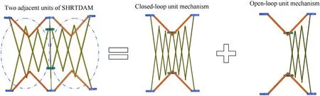
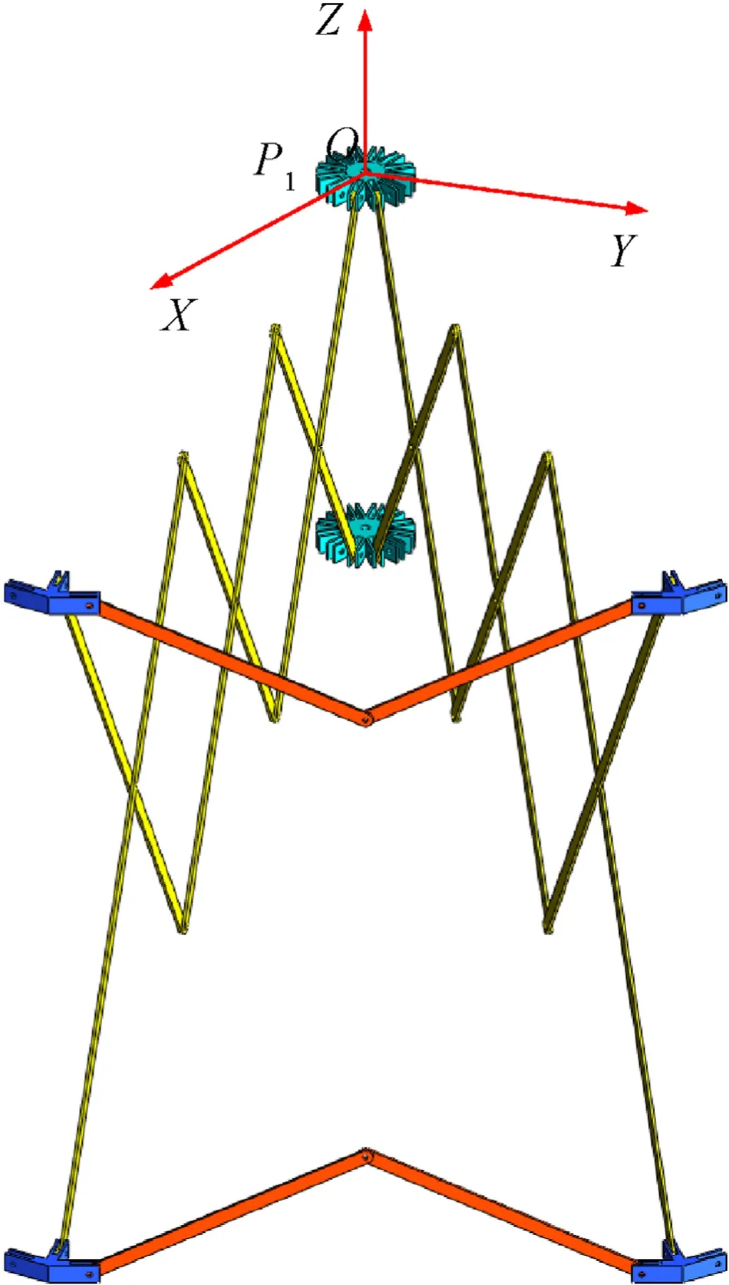
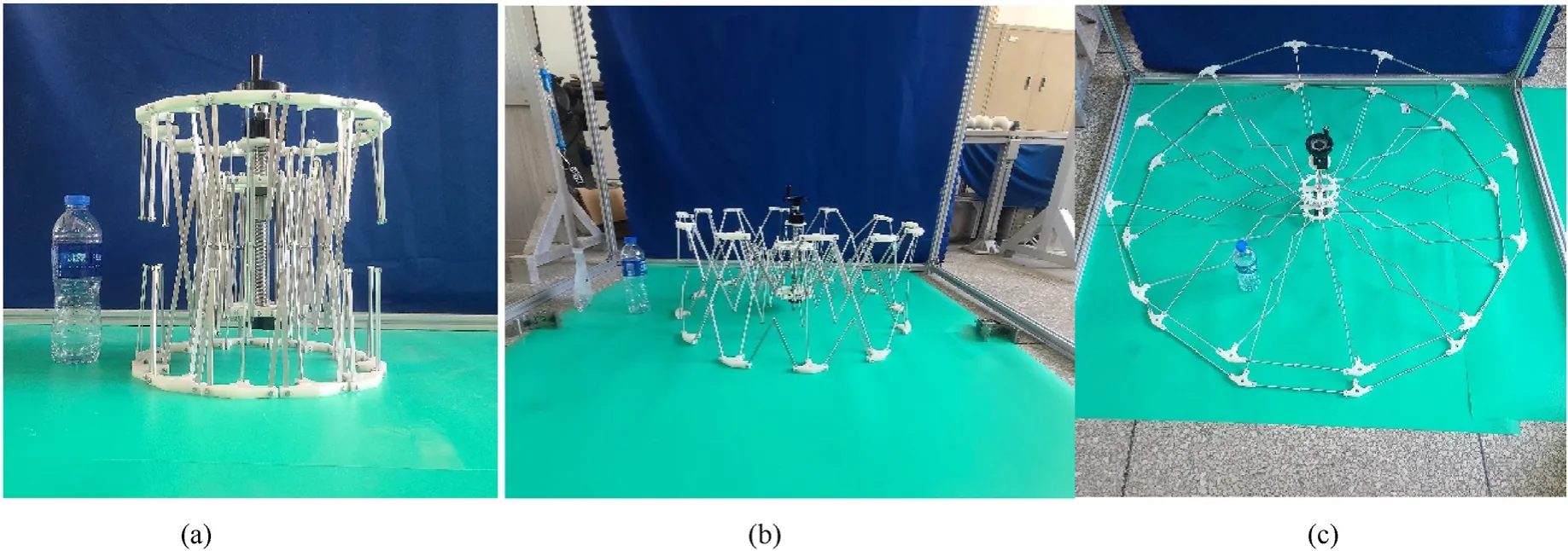
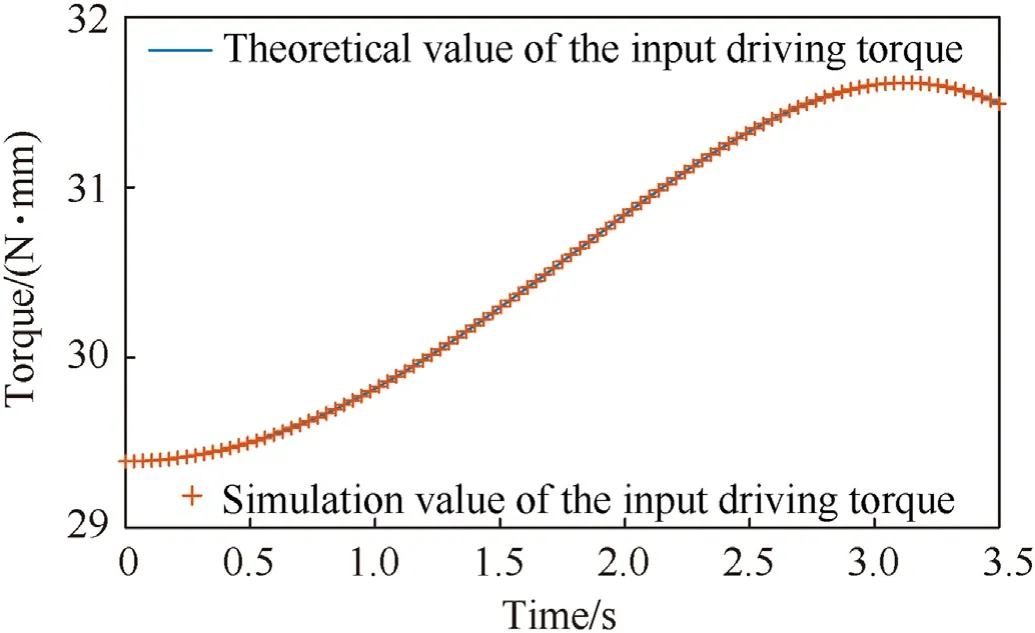
The distance between the rotation axis and the inner node center,as well as that between the rotation axis and the outer node center are set as m. The lengths of the scissor rods at the different levels areL1,L2,L3,andL4,whereL1 As it can be observed in Fig. 4, the vertical projection of the SHRTDAM is a regular polygon with diagonal lines. The projection of each unit mechanism is an isosceles triangle, and the angle between the two waists of the triangle is α. Fig. 4. Vertical projection of the SHRTDAM and its folding process. Based on the size of each component and the angular relationship between components, the relationship between α,θ, and φ is as follows: The SHRTDAM can be decomposed into several triangularshaped units. The adjacent units are connected by an inner node,an outer node, and a rib comprising three sets of scissors mechanisms, all units share two inner nodes. Therefore, the SHRTDAM containsNunit mechanisms, which can be further divided into a closed-loop deployable unit mechanism andN-1 open-loop deployable unit mechanisms (Fig. 5). Fig. 5. Splitting unit of SHRTDAM. The SHRTDAM can be regarded as a combination of closed-and open-loop deployable unit mechanisms. The basis for the DOF analysis of the SHRTDAM is the DOF analysis of the closed-loop unit mechanism. To this end, in this subsection, a closed-loop unit mechanism is selected to perform the DOF analysis. Taking the centroid of the node P1as the originO,the direction of theX-axis is parallel to the rotation axis of the three central rotational joints of a rib, the direction of theZ-axis is vertical upward, and that of theY-axis is determined by the right-hand rule.On this basis, the Cartesian coordinate system of the closed-loop unit mechanism is established (Fig. 6). Fig. 6. Cartesian coordinate system of the closed-loop unit mechanism. According to screw and graph theories, the component is represented by a circle,that is,the nodes are denoted by capital letters,and the chord rods are denoted by the letter X plus numbers.Moreover, the rotational joints between the components are represented by lines, and the rotational line vectors are distinguished by different subscript numbers. This way, the screw constraint diagram of the closed-loop unit mechanism can be established and is illustrated in Fig. 7. Screw theory is used to describe the motion of joints.Taking as an example the rotational joint 5 which connects scissors X11and X12(Fig.7),the twist of the rotational joint 5 can be determined as follows: Similarly, the twists of the other rotational joints can be obtained via screw operations.Since the scissors mechanisms on each rib are the same, the twist on other ribs can be obtained quickly via coordinate transformation. Taking the rotational joints 5 and 16 as examples,it can be found that they have the same position on each rib and the angle between the two ribs is 30◦, thus, the rotational axis direction of the rotational joint 16 is Similarly,the spatial position and the twist of the rotational joint 16 can be obtained easily, consequently, all twists of the closed-loop unit mechanism can be obtained. As shown in Fig. 7, in loop I, the node P1is taken as the fixed platform, the node P2is taken as the moving platform, the following equation can be obtained based on the screw theory: The arrows pointing in the counterclockwise direction as positive, as a result, the above equation can be written as Similarly, for the seven closed-loops (I—VII) in Fig. 7, the corresponding equations can be established as the screw constraint equations of the closed-loop unit mechanisms. where ωidenotes the scalar angular velocity of the rotational jointiin the closed-loop unit mechanism,and0represents a null matrix vector with 6 rows and 1 column. As for the two redundant 3R planar mechanisms on the outer ring truss, the two outer chord rods perform the opposite movement around the common rotational joint, and their steering is opposite. The relationship of the angular velocity between the outer chord rods is Eqs. (6) and (7) can be written in a matrix form as where M represents the screw constraint matrix of the closed-loop unit mechanism, N represents a matrix composed of the scalar angular velocities,and0′represents a null matrix with 42 rows and 1 column. The matrix M can be expressed by 28 column vectors as Therefore,all 28 columns of the matrix M can be expressed as The matrix N can be expressed as The screw constraint matrix M contains 42 rows and 28 columns. The DOFs of the closed-loop unit mechanism can be determined by solving the zero-space dimension of the screw constraint matrix M. By introducing all twists into the MATLAB software, the rank of the matrix M can be calculated as The number of columns of the matrix M is 28,thus,the DOFs of the closed-loop unit mechanism are 28—27=1,i.e.,the closed-loop unit mechanism has only one DOF of retractable motion. According to above analysis,the SHRTDAM can be divided into a closed-loop unit mechanism and multiple open-loop unit mechanisms.When a closed-loop unit mechanism and an open-loop unit mechanism are combined together, a double-closed-loop mechanism is formed. The projection diagram of the double-closed-loop mechanism on the horizontal plane is two isosceles triangles with a bevel. The combined unit mechanism and its coordinate system are depicted in Fig. 8. Fig. 8. Double-closed-loop unit mechanism: (a) Closed-loop unit mechanism; (b) Open-loop unit mechanism. The mechanism on the left side of the combined unit mechanism is the closed-loop unit mechanism exhibited in Fig. 8, while the open-loop unit mechanism is on the right side.The coordinate system is the same as that established by the closed-loop unit mechanism, which is also the global coordinate system of the SHRTDAM.Similarly,based on screw and graph theories,the screw constraint diagram of the open-loop unit mechanism can be obtained (Fig. 9). The components where the open-loop unit mechanism overlaps with the closed-loop one and the corresponding joints are represented by the dotted circle. It can be observed that the shared components are two outer nodes and a rib. Fig. 9. Screw constraint diagram of the open-loop unit mechanism. According to Fig.9,there are seven closed loops(I—VII)in total,thus,seven screw constraint equations can be obtained.The screw constraint equations of the open-loop unit mechanism are where ωidenotes the scalar angular velocity of the rotational jointiin the open-loop unit mechanism, and0represents a null matrix vector with 6 rows and 1 column. Since there are also two redundant 3R planar mechanisms in the open-loop unit mechanism, i.e., similar to Eq. (7), the relationship of the angular velocity between the two outer chord rods is as follows: Eqs. (13) and (14) can be written in a matrix form as where M′represents the screw constraint matrix of the open-loop unit mechanism, N′represents a matrix composed of the scalar angular velocities,and0′′represents a null matrix with 42 rows and 1 column. The matrix M′can be expressed by 28 column vectors as Thus, all the 28 columns of the matrix M′can be expressed as The matrix N′can be expressed as By combining Eqs. (6) and (13), the screw constraint equations of the double-closed-loop unit mechanism can be obtained as follows: Eq. (19) can be written in a matrix form as where In Fig. 8, the rib connected by the nodes P1, P2, C, and D and its 11 rotational joints are shared by two unit mechanisms.In Eqs.(6)and(13),the scissors mechanism and the rotational joints shared by the two unit mechanisms are calculated repeatedly. Therefore, when calculating the DOFs of the double-closed-loop unit mechanism,the twists of the repeated calculations need to be removed,that is,$12to $22should be removed once. Consequently, the screw constraint matrix of the double-closed-loop unit mechanism can be expressed as The matrix P can also be expressed by column vectors as The column vectors in Eq. (23) can be expressed as follows: where042represents a null matrix with 42 rows and 1 column. The rank of the diagonal matrix P is equal to the sum of the ranks of each diagonal matrix(M and M′′),the rank of the matrix P can be obtained as By introducing all twists into the MATLAB software,the rank of the matrices M and M′′can be calculated as Thus, the DOFs of the double-closed-loop unit mechanism can be determined as whereFdenotes the number of DOFs of the double-closed-loop unit mechanism and t denotes the number of columns of the screw constraint matrix P. It is clear that the matrix M′′is a column full rank matrix,Eq.(27)can be written as follows: wheretMdenotes the number of columns of the screw constraint matrix M. According to Eq. (28), the DOF of the double-closed-loop unit mechanism still depends on the matrix M, i.e., the DOF of the double-closed-loop unit mechanism is the same as that of the closed-loop unit mechanism. Based on the previous analysis,it can be understood that,when the open-loop unit mechanism is added on the basis of the combined mechanism(Fig.8),the overall DOF is still the same as that of the closed-loop unit mechanism. Hence, the DOF of SHRTDAM is the same as that of the closed-loop unit mechanism,i.e.,it has only one DOF. The SHRTDAM is a spatially symmetric mechanism,the closedloop mechanism unit can be isolated to perform velocity analysis of the whole SHRTDAM. According to the DOF analysis in Section 3,the closed-loop unit mechanism has only one DOF.Therefore,when an input such as ω1is added to the closed-loop unit mechanism,each angular velocity can be solved via Eq. (6). Based on the geometric parameters of the closed-loop unit mechanism and the screw constraint diagram,the six-dimensional(6D)screw velocity of each node and rod in the closed-loop unit mechanism in Fig. 7 can be obtained through screw algebraic operations. In this paper,the inner node P1is set as the fixed platform,and its motion remains static in the 3D space. The screw constraint diagram of the closed-loop unit mechanism is exhibited in Fig. 7,and the screw velocity of each component in Loop I can be expressed as where0is a null vector with 6 rows and 1 column that represents the 6D screw velocity of each component. In Loop II, the screw velocities of the X11and X12components have been obtained via Eq. (29). Using the obtained screw velocities, the screw velocities of each component in Loop II can be derived as follows: The screw velocity of each component in Loops III-VII can be obtained in a similar manner. According to screw velocity, the angular velocity of each component is where ω(Vi) represents the first three elements of the screw velocity. The centroid linear velocity of each component can be expressed as where v(Vi)is a vector that represents the last three elements of the screw velocity and riis a vector from the coordinate origin to the centroid position of componenti. Since the entire SHRTDAM is a fully centrosymmetric mechanism, the components in each closed-loop unit mechanism have exactly the same size. Moreover, the center of the inner node is centrosymmetric,if a self-coordinate system is established in each unit mechanism, the components with the same position in each unit mechanism will have the same velocity in the self-coordinate system. As it can be seen in Fig. 8, the coordinate systemO-X1Y1Z1is established at the same position of the right open-loop unit mechanism referring to the left closed-loop unit mechanism and the coordinate systemO-XYZ. Since the origins of the two coordinate systems are the same, the velocity of the node C in the coordinate systemO-XYZand that of the nodeEin the coordinate systemO-X1Y1Z1are the same. The corresponding relationship regarding the velocity of the other components in Fig. 9 is similar to that between the nodes C and E, in this way, the velocity relationship can be transmitted to the entire SHRTDAM. Assuming that the entire SHRTDAM has N closed-loop unit mechanismsintotal,thenNcoordinatesystemsO-XYZ~O-XN-1YN-1ZN-1can be established.O-XYZis set as the global coordinate system, the remaining coordinate systems are relative coordinate systems.As shown in Fig.10,the rotation angle between adjacent coordinate systems around theZ-axis is α. In the global coordinate systemO-XYZ, the velocity of each component can be expressed as follows: whereirepresents the number of components andjrepresents the number of coordinate systems. The rotation transformation matrix in Eq. (34) is defined as Through the above analysis,the angular and linear velocities at the centroid of each component in the entire SHRTDAM can be derived and expressed in the global coordinate system through coordinate transformation. The screw acceleration can be determined by deriving the generalized velocity of each component based on the screw derivative. The screw acceleration equation is as follows: where Aidenotes the screw acceleration of componentiin the SHRTDAM,and represents the 6D acceleration column vector of the coincidence point with the origin of the componentireference coordinate system, εirepresents the angular acceleration of the coincidence point with the origin of the componentireference coordinate system,and a is the linear acceleration at the centroid of componenti. According to Eq.(36),in the 6D screw acceleration of componenti, the first three elements are its angular velocity, while the last three elements are its linear acceleration minus its centripetal acceleration. According to the screw acceleration, the acceleration of the inner node P2in Loop I of the screw constraint diagram in Fig.7 can be derived via theLieoperation [ ] as follows: whereP1εP2denotes the angular acceleration of component P2relative to the component P1.The expressions of the two Lie[]are as follows: By combining Eqs. (37) and (38), the following equation can be obtained: where 0 is a null matrix with 6 rows and 1 column. The acceleration screw constraint equations of Loops II—VII in Fig.7 can be obtained in a similar manner.Given the input angular acceleration ε1, the screw acceleration of each component can be calculated using the acceleration screw constraint equations. When the screw acceleration of each component has been calculated, the angular and centroid linear accelerations of each component can be obtained based on Eq. (36) as follows: where ε(εi$i)denotes the origin of the screw acceleration,which is represented by the first three elements, and a(εi$i) denotes the dual part of the screw acceleration,which is represented by the last three elements. Similar to the velocity analysis, all components that have the same position in each unit mechanism have the same acceleration in their own coordinate system. This can be represented in the global coordinate system as follows: Through the above analysis, the angular and centroid line accelerations of each component in the SHRTDAM can be calculated in the global coordinate system. The SHRTDAM has one DOF,the mechanism has only one set of independent generalized coordinates. To simplify the calculations,the angle between chord rods is set to 2φ,and that between scissors at all levels is set to 2θ. The input angle φ is selected as the generalized coordinate, and the dynamic equation can be established according to Lagrange equation as follows: whereEV,EP, andQare the kinetic energy, potential energy, and generalized force of the SHRTDAM, respectively. In dynamic analysis, the clearance and friction of the moving joints are ignored,Qis the generalized driving force applied to the SHRTDAM. 5.2.1. Kinetic energy of the nodes In this paper, the upper inner node P1at the central position is fixed to facilitate the dynamic analysis. According to the above analysis, the rest of the nodes perform the translational motion.Assuming that the mass of the inner nodes ismH1and that of the outer nodes ismH2, the kinetic energy of the nodes can be expressed as follows: 5.2.2. Kinetic energy of the scissors mechanisms In the SHRTDAM, there are 12 inner scissors rods connected to the fixed node, and their kinetic energy can be expressed as whereJ1represents the rotational inertia of the inner scissors rod connected to the fixed node andm1represents the mass of the inner scissors rod. The remaining scissors rods, which include 12 inner scissors rods, 24 middle scissors rods, and 24 outer scissors rods, perform plane motion.The kinetic energy expressions are given below. The kinetic energy of 12 inner scissors rods can be calculated as whereJ2represents the rotational inertia of the inner scissors rod andΟν1denotes the centroid velocity of the inner scissors rod in the global coordinate system. The kinetic energy of the 24 middle scissors rods can be calculated as whereJ3=m2(L2+L3)2/12 represents the rotational inertia of the middle scissors rod andΟν2denotes the centroid velocity of the middle scissors rod in the global coordinate system. The kinetic energy of the 24 outer scissors rods can be calculated as whereJ4=m3(L3+L4)2/12 represents the rotational inertia of the outer scissors rod andΟν3denotes the centroid velocity of the outer scissors rod in the global coordinate system. Therefore,the kinetic energy of the remaining scissors rods is 5.2.3. Kinetic energy of the chord rods In the SHRTDAM,there are in total 48 chord rods,which perform the composite motion. Their kinetic energy can be calculated as follows: The Potential energy and generalized driving forces are both set as 0 in this paper. The velocity of each component can be determined based on the analysis in Section 4 and the dynamic equation of the SHRTDAM can be obtained by substituting Eqs. (43)—(50) into Eq. (42). Thus far, the dynamic model of the SHRTDAM has been established. A novel deployable antenna mechanism named SHRTDAM, has been designed via the variant scissors mechanism, and its kinematic and dynamic have been analyzed. Due to the error between the theoretical analysis and the feasibility condition of the antenna mechanism,the correctness of the theoretical analysis needs to be verified. The SHRTDAM proposed in this paper is composed of too many components. Thus, the analysis and calculation of the dynamic model would be very complex. As a result, computer simulation is an inevitable choice for analyzing the SHRTDAM. For the established model, it is necessary to verify that the simulation model is correct.The Adams/View module provides the function of model verification, which can check the constraints,DOFs, and drive of the SHRTDAM. After the constraints of the imported SHRTDAM model have been created in Adams/View, it is verified that the DOFs of the antenna mechanism are one. Another method that can be used to verify the DOFs of the SHRTDAM is motion simulation.In Section 3,it was found the DOFs of the mechanism are one, the mechanism needs only one drive. The driving angle function is added to the chord rod,as well as the simulation time and timestep size are set to simulate the deployment process of the mechanism. The simulation model of the mechanism is illustrated in Fig.11. Fig.11. SHRTDAM simulation model. After adding one drive, the SHRTDAM can move up throughAdams/motionsimulation and complete the deployment process from the folded configuration to the deployed one. This process is depicted in Fig.12. Fig.12. Simulation of the deployment process in the Adams software: (a) Folded state; (b) Deploying state; (c) Deployed state. The motion of the antenna mechanism is analyzed. When only one drive is added,the motion form of the antenna mechanism can be determined, indicating that the antenna mechanism has only one DOF. This proves that the previous theoretical analysis on the DOFs of the mechanism is completely correct. To further verify that the SHRTDAM has one DOF, a ground experiment prototype of 1.5-m diameter was fabricated and a deployment test is conducted. As shown in Fig.13, the main components include five parts:first-level scissors-like linkages,secondlevel scissors-like linkages, three types of different nodes, and 3R linkages.Considering the inevitable errors in the assembly process,a ball screw pair was selected to drive the mechanism. The deployment process is illustrated in Fig. 14. The deployment test proved that the mechanism has only one DOF and can be deployed smoothly and continuously. Fig.13. Prototype components. Fig.14. 1.5-m prototype: (a) Folded state; (b) Deploying state; (c) Deployed state. In the previous sections,kinematic and dynamic analyses of the theoretical model of the SHRTDAM were conducted, and the theoretical values of each motion parameter were obtained. In order to verify the correctness and feasibility of the theoretical model,the dynamic simulation software Adams and MATLAB were used.Subsequently,the consistency between the results obtained by the two software was assessed. There are several components in the SHRTDAM, and each type of component is located at the same position in each closed-loop unit mechanism. To facilitate the description, in this section, the closed-loop unit mechanism whose own coordinate system coincides with the global coordinate system is selected for the analysis.Taking the closed-loop unit mechanism as an example(Fig.8),the global coordinate system is established at the centroid of the node P1,and the inner scissors rod X13,the middle scissors rod X24,the outer scissors rod X33,the chord rod T1,the inner node P2,and the outer node C are selected for simulation analysis and verification of the theoretical model. Theoretical value calculated by MATLAB software are represented by lines of different colors and simulation value of Adams software are represented by symbols of different shapes. Their displacement, angular velocity, centroid linear velocity,angular acceleration,and linear acceleration of the theoretical and simulation value are presented in Fig.15. Fig.15. Displacement, velocity, and acceleration of the different components: (a) Displacement of the different components; (b) Centroid linear velocity of the different components; (c) Angular velocity of the different components; (d) Centroid linear acceleration of the different components; (e) Angular acceleration of the different components. The curve of the input driving torque of the theoretical and simulation value was obtained as well, and is presented in Fig.16. Fig.16. Input driving torque of the SHRTDAM. By analyzing the motion curves of the inner node P2and the outer node C in Fig.15,it can be found that the angular velocity and acceleration of the inner node P2and the outer node C are both 0.This indicates that, when the SHRTDAM expands from its folded configuration to the deployed one,the spatial motion form of each inner node P2and outer node C in the entire process is translational motion. By analyzing the motion characteristic curves of each component in Fig.15, when only one drive is applied, the motion curve of each component is certain, indicating that the SHRTDAM has only one DOF. The theoretical results in Figs.15 and 16 were consistent with the simulation results,indicating that the relevant motion theory derived above is correct. A new type of deployable antenna mechanism with high reliability and simple structure was proposed in this study, and the kinematic and dynamic characteristics of this mechanism were analyzed, a ground experiment prototype was fabricated and the deployment test was conducted. The experimental results demonstrated the mobility and deployment performance of the proposed mechanism. The highlights of this work are as follows: (1) An ULSM was obtained by changing the position of the central rotational joint of traditional scissors mechanism,based on ULSM, the SHRTDAM with a high reliability and high stiffness is proposed, which can be used as large aperture satellite antenna mechanism. Moreover, a ground experiment prototype of 1.5-m diameter was designed and fabricated and a deployment test is conducted, the deployment test result showed that the mechanism has only one DOF and it can be deployed smoothly and continuously. (2) The motion relationship between the antenna mechanism components was represented as the screw constraint diagram. Subsequently, the screw constraint equations were extracted from the screw constraint diagram, and the number of DOFs of the antenna mechanism was determined by analyzing and solving them. This method relies on matrix operations, which can be applied to solve problems concerning complex mechanism. (3) The kinematic analysis of SHRTDAM was conducted via the screw constraint diagram, the screw and Lie algebraic operations were conducted based on the position of each component in the screw constraint diagram, and through rotation transformation between the coordinate systems,the velocity and acceleration expressions of each component relative to the global coordinate system were deduced. (4) Lagrange equation was adopt to establish the dynamic model of SHRTDAM, the torque required to drive the antenna mechanism was simulated and verified by the Adams and MATLAB software,the results verified the correctness of the dynamic modeling and simulation analysis. In summary, the mechanism proposed in this paper had the characteristic of high reliability and single-DOF,which can be used as a large aperture antenna mechanism,it could also provide a good reference for the design and analysis of large aperture space deployable antennas. Declaration of competing interest The authors declare that they have no known competing financial interests or personal relationships that could have appeared to influence the work reported in this paper. Acknowledgements This work was supported by the National Natural Science Foundation of China (Grant Nos. 52105035 and 52075467), the Natural Science Foundation of Hebei Province of China (Grant No.E2021203109), the State Key Laboratory of Robotics and Systems(HIT) (Grant No. SKLRS-2021-KF-15), and the Industrial Robot Control and Reliability Technology Innovation Center of Hebei Province (Grant No.JXKF2105).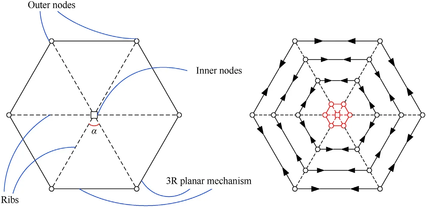
3. SHRTDAM DOF analysis
3.1. DOF analysis of the closed-loop deployable unit mechanism
3.2. DOF analysis of the SHRTDAM


4. SHRTDAM kinematic analysis
4.1. SHRTDAM velocity analysis
4.2. SHRTDAM acceleration analysis
5. SHRTDAM dynamic analysis
5.1. Lagrange equation of the SHRTDAM
5.2. SHRTDAM kinetic energy
5.3. Potential energy and generalized driving forces of the SHRTDAM
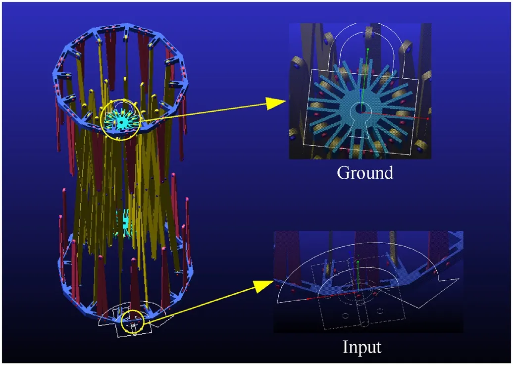
6. SHRTDAM dynamic simulation
6.1. SHRTDAM simulation model analysis

6.2. SHRTDAM dynamic simulation analysis

7. Conclusions
杂志排行

Defence Technology的其它文章
- A review on lightweight materials for defence applications: Present and future developments
- Study on the prediction and inverse prediction of detonation properties based on deep learning
- Research of detonation products of RDX/Al from the perspective of composition
- Anti-sintering behavior and combustion process of aluminum nano particles coated with PTFE: A molecular dynamics study
- Microstructural image based convolutional neural networks for efficient prediction of full-field stress maps in short fiber polymer composites
- Modeling the blast load induced by a close-in explosion considering cylindrical charge parameters