Online asymmetry estimation for whole angle mode coriolis vibratory gyroscopes by high frequency injection

Xiang-rui Meng, Chong Li, Yu-chen Wang

Department of Automation and Measurement, Ocean University of China, Qingdao, 266000, China

Keywords:Rate-integrating gyroscope (RIG)Whole angle mode gyroscope (WAMG)Coriolis vibrating gyroscope (CVG)Online calibration Online identification Online estimation

ABSTRACT

1. Introduction

The rate-integrating gyroscope (RIG), or namely whole angle mode gyroscope(WAMG)operational architecture,is an important operation architecture for the next generation of high performance Coriolis vibrating gyroscopes (CVGs) [1]. It has great potential to conduct ultra-high dynamic measurement range and robust gyroscopes for high-end military applications like spacecrafts [2,3],combat vehicles[4], submarines [5], or tactical missiles [6,7].

The development of WAMGs are motivated by the major limiting factors of the conventional rate output based CVG operation architectures: (1) Bias instability. There are several obvious reasons for this,because the environment of MEMS(Micro-Electro-Mechanical System) gyroscope is not single, the thermal variation has obvious influence on the gyro, which will cause the bias and scale factor drift [8,9]. The naturally occurring flicker noise in the frequency tuned voltage also causes bias instability in the zero rate output of the gyro[10].The stress effect inside the gyro also causes long-term drift of the gyro[11].(2)Dynamic range and bandwidth.It is a very critical problem for quartz CVGs since their dynamics ranges are typically 1◦／s level, though they have admirable bias instability performance. Though micro CVGs are famous for their high bandwidth characteristics,they has failed to meet the state-ofthe-art military applications like high speed spinning projectile[12].The closed-loop control or force-balance mode can effectively improve the bandwidth problem, but the closed-loop gain increases the noise [13]. WAMGs are considered to be the next generation products to overcome these flaws [14], because it can directly measure angle,and has unlimited bandwidth and dynamic range in theory. WAMGs technology can be traced back to 1980s,but it has not become a hot topic until recent years, since the advanced microelectronics allow engineers develop more complicated drive loops [15].

However, the real practice of WAMG also meets several scientific barriers: (1) Stiffness Asymmetry. This refers to the frequency split and the stiffness coupling between the two gyroscopic modes.These errors are mainly caused by the anisotropic properties of materials and manufacturing imperfections, which will result in periodic oscillations in the measurement outputs[16].(2)Damping Asymmetry. Similar to the stiffness asymmetry problem, the quality factors/damping ratios of the two gyroscopic modes are uneven and existing damping coupling terms.It is not a fatal error in the conventional CVG operation, but this will lead the standing wave of the gyro always drift to the lower damped axis, which is extremely severe[16].The damping asymmetry error also can lead to measurement dead area problems. (3) Mixtures between physical rate input and inherent errors. The asymmetry induced errors are difficult to be detected, so develop online calibration methods are challenging [17].

Several solutions have been investigated toward these scientific challenges. Jeffrey Gregory and Khalil Najafi proposed a comprehensive compensation scheme by computing key variables [18].Zhongxu Hu proposed an offline mode matching algorithm for WAMG [19]. Ryunosuke Gando provided a micro controller based one time adjustment to reduce the gyro asymmetry [20]. Kechen Guo investigated a least square approach to estimate the mismatch parameters [21], and his colleague, Yongmeng Zhang, extended to an adaptive gain adjustment method for WAMG [22]. Tsukamoto proposed a novel framework for WAMG based on frequency modulation principle [23]. Due to the environment sensitivity, the offline calibration schemes for WAMG will lose track to the real system. Thus, online calibration scheme is the fundamental solution to conduct reliable WAMG. High frequency injection approaches are effective solutions to estimate/observe unknown values which are widely used in motor control systems. Pascal Combes conducted theoretical research on high-frequency injection and verified the effectiveness of the method through simulation experiments [24]. Bowen Yi proposed a new type of filter applied to the electromechanical systems for the high-frequency signal detection of the dynamic system, and the convergence effect is better [25]. This kind of architectures can inspire MEMS designers and provide an ultimate solution to solve WAMG asymmetry problems.

In this paper, we propose a novel online estimation method to identify WAMG asymmetry errors. The contributions of this work are summarized as follows: (1) A novel high frequency injection based approach is proposed. We introduced a high frequency virtual rotation as a persistent excitation signal for the error identification. The advantage would be that we can separate the physical measurement and error fingerprints with band pass filters to enable online calibration schemes. (2) Proposed effective online estimation algorithms. By numerical solution, we transform the non-ideal differential equation of WAMG into discrete equation,and then design error equation based on this equation.According to the error equation, the optimization scheme is used to track the change of error parameters in real time and realize online estimation. (3) Verified the proposed solution. We select suitable numerical solution and optimization scheme to combine, forming four groups of solutions for comparative experiments. The output angle value of the WAMG is obtained through the simulation experiment of infinitesimal steps, and the error parameters are tracked by using multiple groups of values at the previous and the next moment. Finally, we get the experimental results and verify the most effective online estimation solution under different conditions.

The following paper is a detailed description of the above research content.

2. Theory

2.1. Model of WAMG

The basic principle of WAMG is based on Coriolis force effect.By letting the harmonic oscillator of the gyroscope oscillate freely,the standing wave angle is measured according to the position ofXYaxis, as shown in Fig.1.

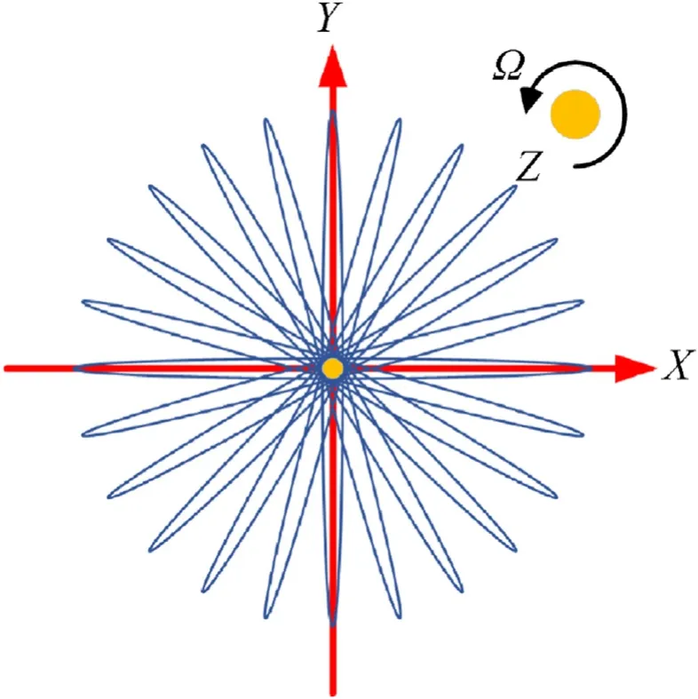
Fig.1. Mass center orbit of the WAMG.

The resonant gyroscope has a set of mechanical suspension in eachXYdirection,and the differential equation modeling onX-axis andY-axis is shown as follows:

wheremis the mass of gyroscope,xandyare the displacements of the gyroscope two modes (Xmode andYmode),cxandcyare the damping coefficients along theXmode andYmode respectively.kxandkyare the stiffness coefficients along theXmode andYmode respectively.Fxis the driving forces on theXmode,Fyis the driving forces on theYmode.

The above equation Eq. (1) is in theXYplane. When physical rotation Ωzis generated on theZaxis perpendicular to theXYplane,the Coriolis force effect will be generated on theXYplane,and then will form “the Gyroscope Effect”. The equations on the above two modes will become as follows:

WAMG requires free oscillation,which means thatFxandFyare both zero in two modes. The above equation Eq. (2) can be solved by means of average method, and the solutions in the two modes are as follows:

whereais the amplitude of the vibrations determined by the initial condition ofx（0）andy（0）,θ0is the initial standing wave angle,ωxis the resonant frequency along theXmode, ωyis the resonant frequency along theYmode.

2.2. Angle dynamics

Under ideal case, the damping and stiffness of resonant gyroscope are highly symmetric (cx=cyandkx=ky), and the free response equation of the WAMG is

where ˙θ is the standing wave angle,kis angular rate gain, Ωzis physical input angular rate.

Due to the limitation of materials and processing, it can't achieve the complete consistency of damping and stiffness in the two modes. Under the non-ideal case, the response equation of the WAMG will be rewritten as follows:where Δ（1／τ） is the damping inconsistency error, Δω is the frequency asymmetry error,Qis the quadrature error,Eis oscillation energy of the gyroscope.

The main reason that the WAMG cannot measure the integrated rate accurately would be the presence of asymmetry of damping coefficient and the inconsistency of stiffness coefficient between the two modes. They can affect the output angle of the gyroscope and cause the problem of high threshold. In order to overcome periodic oscillations and measurement dead area, finally achieve the complete free response of the harmonic oscillator, the consistency of the two modes should be improved as much as possible.The actual environment in which gyroscopes are used is unstable and affected by temperature and humidity,sok,Δτ and Δω are not constant and will change constantly under the influence of the environment. Therefore, it is an important research problem to adopt reliable online methods to estimate asymmetry in real time.

2.3. Problem foundation

Based on the above non-ideal dynamic model of WAMG standing wave angle,the WAMG online identification and tracking method is designed to solve the following two problems:

(1) Identify the error parameters of WAMG. According to the non-ideal dynamic model Eq.(5),the error parameters to be identified by the identification method include angular rate gain, damping asymmetry error and frequency asymmetry error, and they are time-varying parameters.

(2) The process of identifying error parameters does not affect the normal operation of WAMG.The task of the WAMG is to detect the standing wave angle of gyroscope, and it can be continuously obtained by detection. The identification method requires that not only the variation of standing wave angle caused by physical rotation,but also the gyro response with error information can be obtained.

In order to solve the above problems, we propose an online identification method of WAMG with high-frequency injection.The details of this work are described in the following chapters.

3. Methodology

3.1. Novel online driver

The novel WAMG system architecture with virtual electric rotation is composed of the online driver and the online estimator as illustrated in Fig. 2.

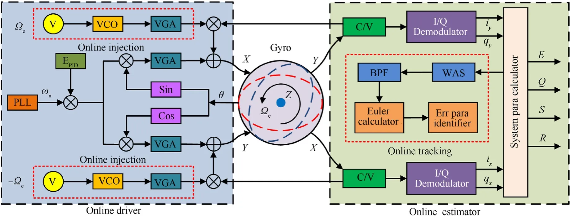
Fig. 2. Novel online driver and online estimator architecture.

The online driver includes: phase-locked loop (PLL), variable gain amplifier (VGA), voltage source (V) and voltage controlled oscillator(VCO).The gyroscope is driven at the resonant frequency by the PLL.The total oscillating energy is maintained with a value of(EPID).This control loop compensates the damping induced energy dissipation while maintain the oscillation in a free standing wave manner.

The essence of virtual electric rotation is to simulate Coriolis forces. This simulated Coriolis forces are generated electrically without introducing external physical rotation. We introduce electric Coriolis force by introducing permanent high frequency signal into the driving circuit equivalent to electric rotation excitation. The form of virtual rotation Ωeis shown aswhereA0and ωeare the amplitude and frequency of virtual electric rotation respectively.

The virtual rotation is generated by voltage sources, VCO and VGA.We use the driving signal formed by the superposition of high frequency injection and energy control to actuate the gyro. The high frequency excitation scheme is added in the driving circuit,and the high frequency excitation signal can be added independently in the two modes. According to the gyro dynamics, Ωeis introduced in theXmode, and theYmode is - Ωe. The output signals of two modes of gyro are mixed with high frequency excitation signals.In this way,it can ensure that the frequency of input high frequency excitation signals is the resonant frequency of the gyro.

When virtual electric rotation is added, the Coriolis force differential equation Eq. (2) on the two modes of the gyro is transformed as follows:

According to the current gyro differential equation Eq. (7), the dynamic output response equation of WAMG in the non-ideal case is rewritten as follows:

wherefqsis the control input force of virtual electric rotation,fqs=kΩΩe,kΩis the electric gain of virtual electric rotation.

3.2. Novel online estimator

The online estimator includes:current to voltage(C/V)amplifier,I/Q demodulator,system parameters calculator,whole angle solver(WAS), band pass filter (BPF), Euler calculator (EC) and error parameter identifier.The C/V circuits are used to amplify the highfrequency output gyro signals. Then the I/Q demodulator extracts the signals of the two modes of the gyro into four parametersix,qx,iyandqy. By using the gyro system data processor, which can also be called para calculator, we can get four calculated parametersE,Q,RandSas

whereRandSare used to calculate the standing wave angle of the gyroscope. According to the calculated parameters, the standing wave angle θ can be obtained by using WAS

The calculated standing wave angle is used to distribute the excitation energyEPIDas described above.

The angular response is decomposed into high-frequency and low-frequency parts by BPF, and the high-frequency part is the response corresponding to high-frequency injection. Finally, the obtained gyro standing wave angle response output is the gyro response generated by the virtual electric rotation after filtering the low-frequency physical rotation, and its form is shown as follows:

The Euler calculator uses Eq. (11) to perform difference calculations to constructing error equation for the error parameters identifier. Section 3 gives details.

3.3. Novel online tracking approach

The proposed method includes the following stages as shown in Fig. 3: (1) The virtual electric rotation is injected into the gyro online in the form of a high-frequency signal.(2)The gyro produces a corresponding standing wave response in the high frequency band, which can characterize error parameters. (3) Through the well-designed I/Q demodulator, WAS and BPF, the system realizes the online fast extraction of the virtual electric rotation response.(4) The Euler calculator and error parameters identifier that are fully designed for the gyro implement online tracking of the error parameters.

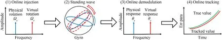
Fig. 3. Novel online high frequency excitation and online tracking process.

The remainder of this section gives the details.

3.4. Euler calculator

Under high frequency excitation, the ideal equation Eq. (4) can be simplified, and the equation is shown as follows:

where α1represents virtual angular rate gain, μ is the virtual rotation, i.e. Ωe, which is a new notation defined for clear mathematical expression.The response signal of gyroscope is introduced by actual physical rotation and high frequency virtual electric rotation, which can be separated by filter.

The above non-ideal equation Eq. (5) is also simplified for modeling, and the equation is shown as follows:

where α2represents the error term introduced by damping inconsistency, α3represents the error term introduced by the frequency mismatch of the two modes.

For the WAMG system,the standing wave angle can be detected all the time, and the virtual electric rotation is the given term.Therefore, the above differential equations can be solved numerically by discretization method. There are two solutions: Euler method (EM) and Forward and Backward Euler method (FBEM).The latter is also called the second-order Runge-Kutta method(RK2)or predictor-corrector Euler method.Based on the non-ideal gyro response model, the Euler calculator is constructed as Euler method:

Forward and Backward Euler method:

where θn,θn＋1,μn,μn＋1are known values,his the step simulation length.

3.5. Error equation

The error equation is constructed by the above numerical solutions. According to this equation, we can identify the error parameters α1, α2and α3by the optimization methods. The error equation is shown as

wherexmeais the measurement at the next moment,xcalis a numerical solution calculated by Euler calculator according to the measured value at the current moment.

According to Eq. (16), the error functions of the two numerical solutions are constructed.The characteristic of the WAMG is able to directly measure the angle θ of the gyroscope,and the angle value can be continuously obtained. According to the measured angel value θnat current moment, we can use the method of numerical solution to calculate the angle value at the next moment. The interval between the current moment and the next moment is the unit steph. Then we make the difference between the angle value measured at the next moment θmeaand the calculated value θECcalto get the error function. The θECcalcontains two methods of calculation, i.e. θEMcaland θMEMcal. The two error equations constructed by Euler method and Forward and Backward Euler method are shown as follows:

Euler method:

Forward and Backward Euler method:

The error equation has to be deformed to make the optimization more traceable. Their equations are shown as follows:

whereMis a matrix related to μ, sine and cosine functions. α =[α1, α2, α3］T.

In order to apply the following optimization method,we need to transform it as follows:

3.6. Error parameters identifier

In order to accurately identify the parameters of the error term with the least amount of data in a short time, it is particularly important to choose the appropriate optimization method for unconstrained problems.

The most common optimization method is gradient descent method. The descent direction of it is the negative direction of gradient, i.e. -λ∇f（αk）. It has the following form:

where αk＋1is the matrix of parameters to be identified at the next moment, αkis the matrix of parameters to be identified at the current moment,λ is the step size of the current moment,∇f（αk）is the direction of the gradient at the current moment.

Traditionally,the negative direction of the gradient indicates the direction of the fastest descent.The step size λ of gradient descent method needs to be manually adjusted for many times.We have to find the step that can achieve the fastest descent speed and reach the convergence position as quickly as possible. Therefore, this method is not adaptable to gyroscope in different environments.

The rule of steepest descent (SD) method is to update the descent step size of each iteration by using the matrixM. It can automatically update the step size λkand its update mode is shown as

where λkis update the step size of SD at the current moment.

The descent direction of SD is also the negative direction of the gradient. Thus,the SD has the following form

It can achieve the effect of shortening the number of iterations compared with the traditional gradient descent method but increasing the amount of computation for each iteration descent.

The rule of conjugate gradient(CG)descent method updates the descent direction and step size.First of all,we calculate the gradient direction of the first step, it is shown as:where γ0is the initial residual, which is the initial gradient direction off（α）,η0is the first descent direction of CG.

If the first gradient is not zero(γ0≠0),the CG continues the loop(k= 0,1,2…) until it converges. And then, we calculate the step size δkand update the step size of each iteration,it is shown as:

where δkis the updated step size of CG at the current time,γkis the residual of the current moment,ηkis the direction of descent at the current moment.

Finally,it can descend in the direction of the conjugate gradient.The CG has the following form:

The formulas from Eq. (27) to Eq. (28) are used to correct the negative direction of the gradient, and the search direction of the previous step ηkis retained, and it is used to form the conjugate direction, which becomes the next direction ηk＋1.

Before calculating the conjugate direction at the next moment,we need to calculate the gradient direction at the next moment γk＋1, which is the residual at the next moment. Its form is shown below:

where γk＋1is the residual at the next moment.

The CG only needs to use the last conjugate vector ηkto find each conjugate vector ηk＋1,and does not need to remember all the previous conjugate vectors. The new direction used in each iteration is a linear combination of the negative residual at the next moment-γk＋1and the previous direction of descent ηk.It is shown as

where ηk＋1is the direction of descent at the next moment.

The coefficient βkcan be obtained according to the conjugate condition (ηTkMηk＋1= 0). Its form is shown below:

where βkis the coefficient used to compute the conjugate direction.

In this way, the descending direction after each iteration is the conjugate direction. This method has fewer iterations, but more computation in each iteration.

Therefore, we get four online estimation methods to identify three error parameters at the same time, i.e Euler method combined with the steepest descent method(EM ＋SD),Euler method combined with the conjugate gradient descent method(EM ＋CG),Forward and Backward Euler method combined with the steepest descent method (FBEM ＋SD) and Forward and Backward Euler method combined with the conjugate gradient descent method(FBEM ＋CG).The four methods are used to identify the variation of three error parameters α1,α2and α3.

4. Validation

4.1. Preliminary parameter measurement

In order to improve the accuracy and authenticity of the experiment, it is necessary to measure the related parameters of the gyro and calculate the initial values of the error parameters to be identified.To this end,we designed and implemented a WAMG test board as shown in Fig. 4. The gyroscopes of the same batch have been tested to get the following approximate parameters as shown in Table 1.

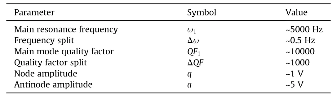
Table 1The approximate parameters of the measured gyros.

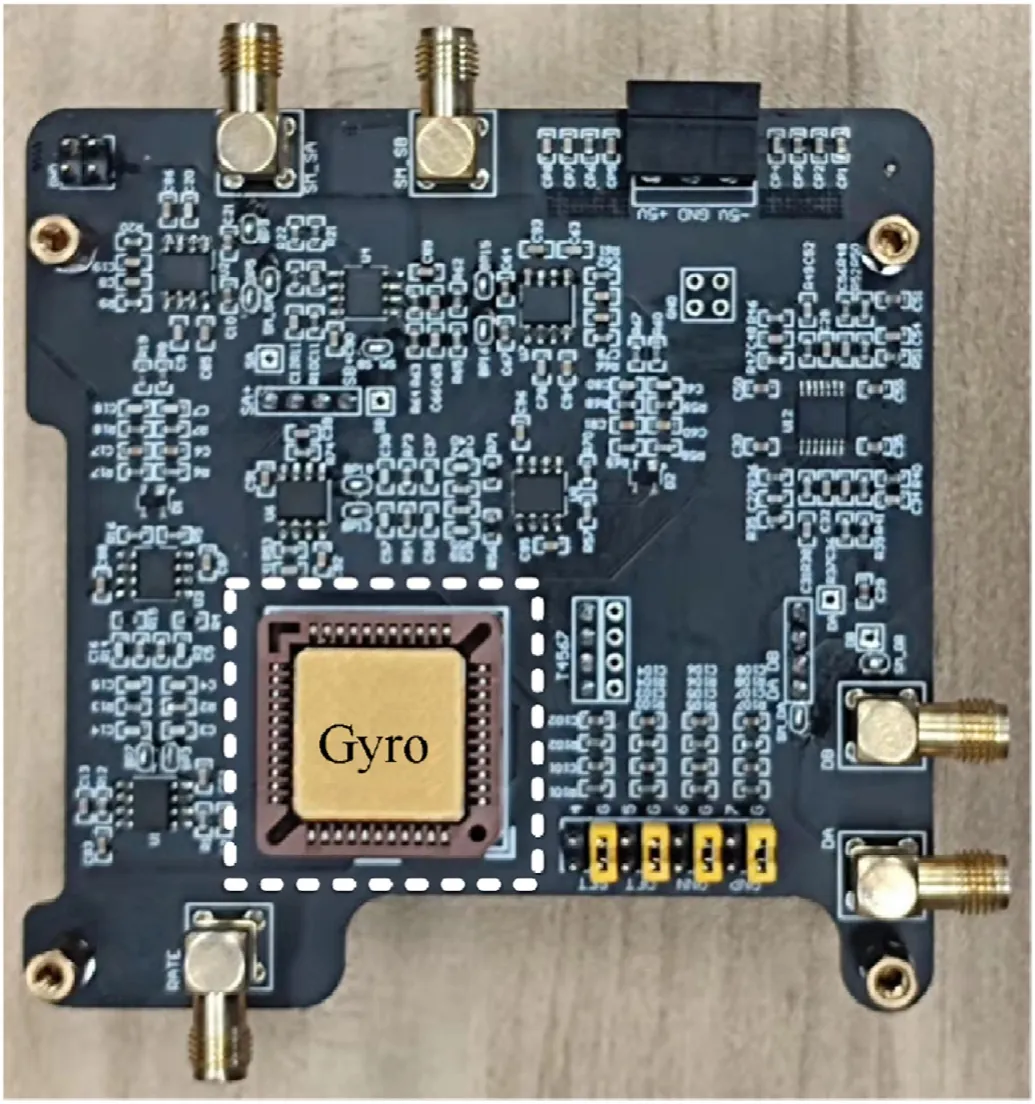
Fig. 4. The WAMG test board for measuring gyro parameters.

The following equation can be derived by Eq. (5):where Δω = ω1- ω2, i.e. the difference between the main resonance frequency and the secondary resonance frequency. ΔQF=QF1-QF2, i.e. the difference between the quality factors of the main and secondary modes.keis the circuit gain parameter variable that can be customized.

Note that the resonant frequency is calculated in the form of angular frequency in rad,andQ／Eis dimensionless. According to Table 1 and Eq.(30),the nominal initial value is α =[-1 0˙2 0˙5］ㅜ.In the same initial conditions, we carry out the comparative experiment. This can ensure the accuracy of the experimental verification scheme and make the experimental results more convincing.

4.2. Comparison of euler calculator

The effectiveness of the Euler calculator is the basis and premise of the reliability of the error parameter identifier. This subsection compares and evaluates the two schemes of Euler Calculator.Simulation experiments are carried out in MATLAB 2020b.

The μ is the input signal and represents the virtual electrical rotation.Its frequency is higher than the ordinary physical rotation.We set μ as a sinusoidal signal with the frequency of 50 Hz (100 π rad).In this way,the simulation experiment can be more realistic.

In order to accurately evaluate the effectiveness of the Euler calculator, it needs to design experiments to generate standard truth values. When the simulation step size is small enough, the simulation value of the every step can be regarded as the standard true values.The simulator is built based on high-order models and infinitesimal step sizes to ensure practicality. The total simulation time is set to 10 s, and the simulation step size is 10-5s.

According to the simulation true value of each step, the angle value of the next step is calculated by the above two Euler solutions.By comparing the results calculated in the next step with the truth value, the accuracy of the two methods can be obtained. The transient results are biased, so we extract the steady-state results over a period of time for comparison as shown in Fig. 5.

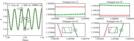
Fig. 5. Accuracy of two numerical solutions of the Euler calculator.

The curves of the two methods basically coincide with the true value curve,which shows that the two methods have high accuracy.It can be seen in the partial enlarged view that FBEM has higher accuracy at the lowest and highest points of amplitude. On the biased baseline, the two methods are equally comparable. We can see that although the calculation process of EM is relatively simple,its accuracy is not always lower than that of FBEM.

4.3. Experiment setup

In actual MEMS gyroscopes, since these three parameters to be identified are all slowly varying variables with respect to time,there is no need for high identification frequency.Therefore,we set the identification frequency to 0.1 s, which means that parameter identification is performed every 0.1 s. The four error parameter estimation methods identify the three parameters simultaneously.They start and stop at the same time.

The total amount of simulation data within 10 s is 106.However,the actual microprocessor cannot achieve such a high acquisition rate. For more realism, we use the down-sampling method to set the number of acquisition points per second to 1000.It is assumed that the initial set point before tracing is α =[-2 1 1］ㅜ.Because in practice, the error parameters can be estimated, the initial value need not differ much from the standard true value,and the order of magnitude should also be within a reasonable range.

4.3.1. Static test

In order to preliminarily evaluate the performance of the four methods, the static error parameters are first tested, that is, the identified error parameters do not change with time. When the error parameters are static, the judgment stop conditions of the four online identification schemes are consistent for fairness. The iteration is stopped when the error parameter variation is small enough and the number of iterations is not limited.

4.3.2. Dynamic test

In a relatively stable environment,these three errors parameters can remain constant,but they can rarely be achieved.More MEMS gyroscopes are in a variable environment.Therefore,we need to set the parameters to be more consistent with the actual simulation.It is mainly set as slow change and sudden change.In most cases,the change in parameters is abrupt,so we set the abrupt case as sharp linear change and exponential change. The three variations of the three parameters are shown as

(1) 0˙1% linear change:

(2) 10% linear change:

(3) Exponential change:

For the above dynamic case, the three error parameters are changing all the time. The error parameters are identified every 0.1 s, so they are identified 100 times in 10 s. The judgment stop conditions of the four online estimation methods are the same.When the error parameter variation is small enough (<10-6), the identification will stop. The maximum number of iterations for each identification is 1000 for fair comparison. The estimation method track the parameters changes, and deliver the tracking results of each 0.1 s to the next follow-up.

4.4. Experiment results

4.4.1. Static results

In the static test, that is, when the error parameters are stable,all the four estimation methods can realize parameter identification and estimate the approximate parameter truth value,but they are different in accuracy and iteration times.

When the error parameter variation of their judgment stop is set at 10-6, the results are shown in Table 2. EM ＋SD has the largest number of iterations, and EBEM ＋SD has the second number of iterations.The SD method combined with the two Euler calculators cannot effectively shorten the number of iterations.Compared with the CG method,the convergence effect of error parameter α1of the SD coordinated optimization method is not good, and the convergence error is within 4%.The convergence error of the other two error parameters α2α3is less than 1%˙The iteration times of EM ＋CG are consistent with those of FBEM ＋CG, and the identification errors of the three error parameters tracking are very small,which can achieve excellent identification effects.

Table 2The static test results when the convergence judgment stop condition is 10-6.

When the convergence step is set at 10-10, the results are shown in Table 3.The convergence effect of the SD method is better,but the number of iterations is greatly increased.The convergence effect of CG is basically unchanged.

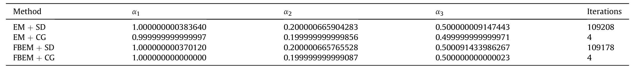
Table 3The static test results when the convergence judgment stop condition is 10-10.

The identification results show that when the error parameters are in the static test,the difference between the FBEM and the EM combined with the optimization method is not obvious, which cannot reflect the superiority of parameter identification. Therefore,further comparison is needed when the error parameters are in the dynamic state.Obviously,the SD method has no advantage in the number of iterations, but because of the simplicity of the iterative process, this method can implement the algorithm in processors with small resources, reduce the occupation of resources,and still has reference value.

4.4.2. Dynamic results

In the dynamic test, that is, when the three parameters are changing dynamically,the results of the four parameter estimation methods are not the same. Because there is a certain difference between the initial value of the set identification error parameter and the real value, the initial parameter identification has special significance. Therefore, we divided the 10 s identification process into two stages. They are the 0 s—2 s rapid identification of parameters and 2 —10 s moderated tracking of parameters. In this way, we can compare the accuracy and rapidity of the four estimation methods of the three dynamic tests more comprehensively.

(1)Identification of0˙1%change:When the three error parameters change 0˙1%within 10 s,their identification process I s shown in Fig. 6. The SD method with two kinds of Euler calculator (EC ＋ SD) cannot track the error parameters quickly within a limited number of iterations,and it achieves a tracking error of less than 0˙1%in about 0.6 s.The tracking effect of 1 s—2 s is good, but the tracking accuracy is worse than CG method combined with Euler calculator (EC ＋CG).The EC ＋CG can quickly track the error parameters,and the three parameters can be traced simultaneously with high precision.In the following 8 s,the four parameter estimation methods has a better tracking effect for error parameter α1.For the tracking of error parameter α2, EC ＋SD has overshoot,but the tracking can continue after 7 s.For the tracking of error parameter α3, although the tracking accuracy of the SD method is relatively low, it has a trend of gradually improving accuracy. In general, within 10 s, the tracking speed of the EC ＋SD is slow and there is overshoot,but the tracking effect of the three parameters is gradually improving. EC ＋CG tracking accuracy is always high.

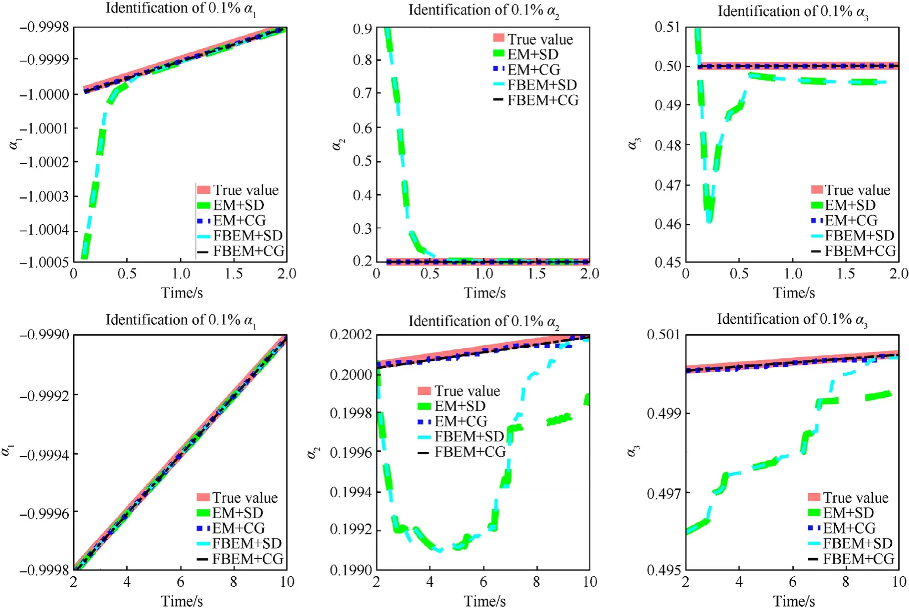
Fig. 6. Tracking of three parameters that change 0.1% in 10 s.

(2)Identification of10%change:When the three error parameters varies by 10% within 10s, their identification process is shown in Fig. 7. For error parameter α1, the four methods can quickly track the error parameter from the beginning,and all can achieve high-precision tracking within 10 s.For error parameter α2,the EC ＋SD in the 0s to 2 s does not achieve rapid tracking, but the accuracy gradually improves. The tracking error after 1.4 s is within a reasonable range,but the EC ＋SD overshoots after 2 s,and the tracking accuracy is always lower than that of EC ＋CG. For error parameter α3, in the 0s to 1.5 s, the EC ＋SD appears overshoot, but then the accuracy gradually improves, and the tracking accuracy is still inferior to EC ＋CG.In general,highprecision tracking can be achieved for error parameter α1within 10s, and overshoot occurs for error parameter α2α3.The accuracy of the EC ＋SD is lower than that of the EC ＋CG.

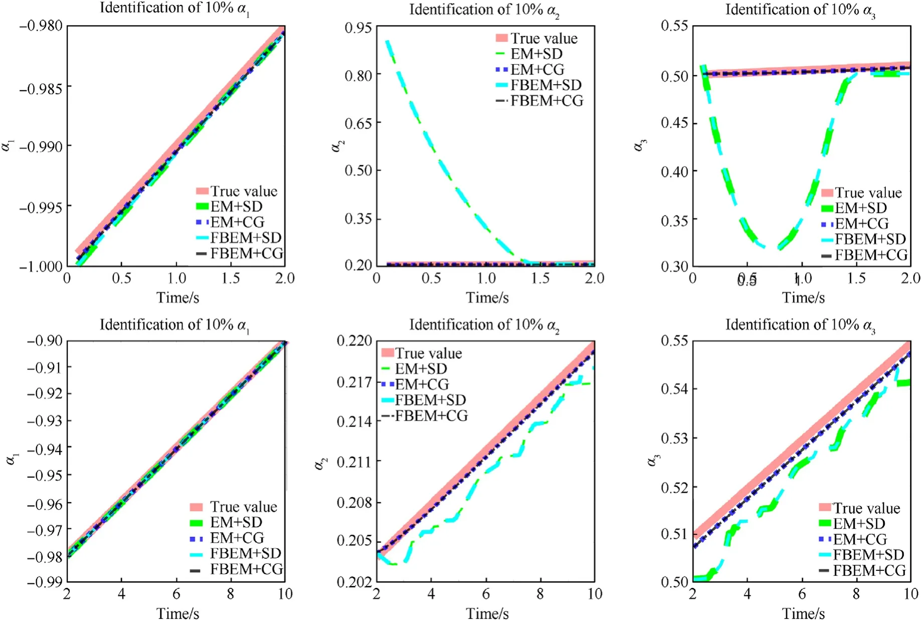
Fig. 7. Tracking of three parameters that change 10% in 10 s.

(3)Identification of exp change:When the three error parameters change exponentially within 10s, their identification process is shown in Fig. 8. For error parameter α1, the four error identification methods can quickly and accurately trace within 10s. For error parameter α2, EM ＋SD has the slowest tracking speed in the 0 s—2 s.After 0.5 s,the tracking accuracy of two estimation methods of Euler method combined with optimization method(EM ＋OM)is similar.In the first 2 s, the tracking effects of the two identification methods corresponding to FBEM are relatively close. In the last 8 s, EM ＋CG has the highest tracking accuracy, while EM ＋SD has the lowest tracking accuracy. The FBEM ＋SD and FBEM ＋CG have similar tracking accuracy and gradually improve their accuracy.For the error parameter α3,EM ＋SD overshoots in the 0 s—0.5 s. After 0.5 s, the accuracy of the two estimation methods of EM ＋OM is close, and the accuracy of the two estimation methods of FBEM ＋OM is close and higher than EM ＋OM. In the next 8s, the accuracy of EM ＋CG gradually improves, and the accuracy of EM ＋SD gradually decreases, but the change of error parameters is still tracked by EM ＋SD.Overall,FBME ＋OM provides faster and more accurate identification. EM ＋CG accuracy gradually improved, EM ＋SD accuracy is not satisfactory.

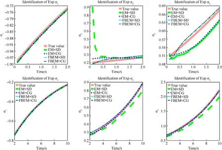
Fig. 8. Tracking of three parameters that change exponentially in 10 s.

4.4.3. RMSE results

Since our estimation method is online and continuous real-time tracking,and the amount of data tracked in a short period of time is large,it is impossible to check a certain value to determine whether the tracking is abnormal, nor can it be judged that the tracking effect of the entire system is poor through a number of abnormalities. We need to comprehensively evaluate multiple continuous tracking effects. Therefore, we use a common evaluation index: root mean square error (RMSE),its range is not limited,the lower the value, the lower the error rate, the higher the tracking accuracy, and it is suitable for parameter estimation tracking experiments with overshoot.Its calculation formula is as follows:

wheremrepresents the number of total samples,αtrue（i）represents the true value of thei-th sample, αpredicted（i）represents the predicted value of thei-th sample.

Since we discussed the parameters tracking of 10 s, we also calculated the RMSE in this section, respectively calculating the RMSE in the parameter rapid identification stage and the RMSE in the parameter moderating tracking stage.

In the 0 —2 s, the differences in different parameter change modes of different identification methods are more obvious, and the difference between them is on the order of 10-2. The differences between them are shown in Fig. 9. When the parameters change slowly, the four online estimation methods have very little difference in the estimation accuracy of error parameter α1,but since the identification of the three parameters is synchronized,when the identification stops, the identification accuracy of EC ＋SD for error parameter α2α3is obviously insufficient. It is mainly because of the limitation of the number of iterations.When the parameters change drastically linearly, the identification accuracy of the EC ＋SD method for error parameter α2is slightly reduced, and the identification accuracy for error parameter α3is significantly reduced.When the parameters change drastically,the tracking accuracy of error parameter α1drops slightly because the change of the parameter is more drastic, but it still remains at a higher level. For error parameter α2α3, EM ＋ OM has lower tracking accuracy than FBEM ＋OM. FBEM ＋SD and FBEM ＋CG have little difference in tracking accuracy.

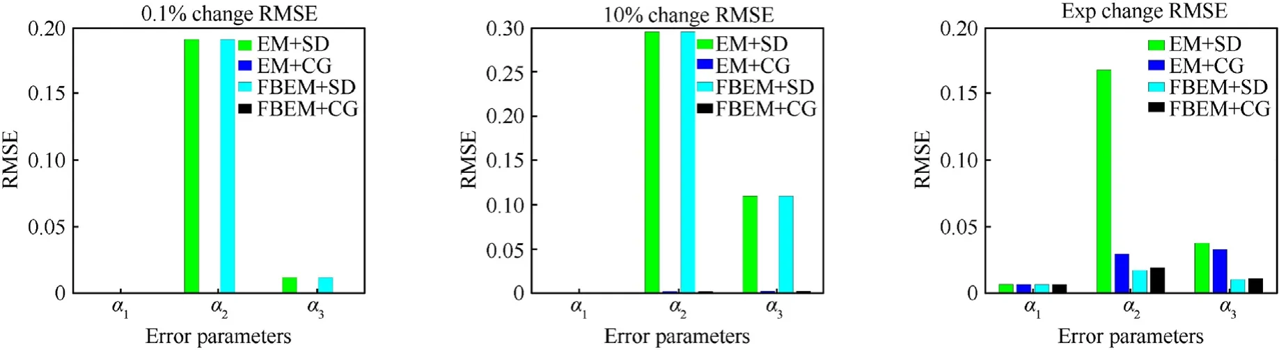
Fig. 9. RMSE of 0 —2 s.

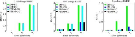
Fig.10. RMSE of 2 —10 s.

In the 2 s—10 s, as shown in Fig. 10, the tracking of the four methods for the three error parameters is reduced to the order of 10-3in the experiment where the error parameters varied slowly and the error parameters varied rapidly.In these two experiments,the tracking accuracy of the four estimation methods for error parameter α1is basically the same, but the tracking accuracy of EC ＋SD for error parameter α2α3is obviously lower than that of EC ＋CG,but their overall accuracy is one order of magnitude lower than that of 2 s ago. This shows that in the last 8s, the tracking of error parameters is more and more accurate. In the experiment of parameters exponential change, the accuracy of tracking results after 8 s does not improve significantly in order of magnitude compared to the experiment 2 s earlier. The tracking accuracy of error parameter α1is basically the same,but the comparison of the tracking results of the other two error parameters is more obvious.The tracking accuracy of FBEM ＋OM is the highest, and the accuracy ratio of FBEM ＋SD is higher than that of FBEM ＋CG in error parameter α2,while the accuracy ratio of FBEM ＋SD is lower than that of FBEM ＋CG in error parameter α3.

4.5. Discussions and suggestions

Based on the above theoretical research and experimental verification,it can be concluded that all the four methods can track the changes of the three parameters, and there is not much difference between their tracking results,but there are still significant differences between them, which can be summarized as

(1) In the case of slow and fast linear variation of error parameters,it is most obvious that the CG method has a significant advantage over the SD method in the accuracy of the error equation composed of the same Euler calculator.

(2) In the case of exponential variation of error parameters, the effect of FBEM ＋OM is better than EM ＋OM.However,there is not much difference between FBEM ＋SD and FBEM ＋CG.

(3) Obviously, the convergence state can only be achieved with more iterations of the SD method,while the CG method can achieve convergence with a very small number of iterations,but every conjugate gradient iteration is more complex.

These three points can help engineers select suitable scheme for parameter tracking, so that error parameters can be effectively tracked in a short time.However,the low number of stacking does not necessarily mean that it is suitable for all practical engineering needs, so here are some suggestions for parameter tracking schemes.

(1) The CG method has the least number of iterations, but each iteration calculation is more complex, which may not be suitable for microcontrollers with small resource utilization,but it is still suitable for high-speed microcontrollers.

(2) The SD method is still recommended when the environment is stable.Although the initial stage of identification requires a certain amount of time to identify, with time going, the accuracy gradually improves, the number of iterations will be fewer, and each calculation is relatively simple.

(3) Even when compared to the true value, the difference between the FBEM and EM is not high.However,in a drastically changing environment,the FBEM has higher accuracy,which is more advantageous than EM in tracking parameters.

Although the structural design optimization,material upgrading and processing technology improvement can promote the symmetry, reduce the bias drift and improve the ZRO stability of gyroscopes, it is not to achieve complete symmetry for a long time.The offline correction scheme can achieve the symmetric state of the two gyroscope modes at the beginning,but cannot achieve the asymmetric parameters remain unchanged over time. It is necessary to use the online correction method to track the change of error parameters in real time.

5. Conclusions

A novel online injection approach is proposed to identify the error parameters of WAMG asymmetry under the non-ideal conditions. An effective online estimation algorithm is then proposed based on this method.The WAMG dynamics are discretized in the form of numerical solution to construct the error function using EM and FBEM.Then they are combined with two optimization schemes to identify error parameters of the WAMG. Through the validation experiment, the proposed method can effectively track the dynamically changing error parameters. According to the comparison results, it is obvious that the CG combined with the two numerical solutions can achieve the fastest convergence speed,and the FBEM combined with the CG can achieve the highest accuracy of tracking effect.The RMSE,that reflects the tracking accuracy,can reach the level of 10-3under the dynamic change of the gyro error.In the future, it is suggested to be applied to the actual WAMG application platform to fully improve performance.

Declaration of competing interest

The authors declare that they have no known competing financial interests or personal relationships that could have appeared to influence the work reported in this paper.

Acknowledgements

This work is funded by the National Natural Science Foundation under grant No. 62171420 and Natural Science Foundation of Shandong Province under grant No.ZR201910230031.