A combined finite element and deep learning network for structural dynamic response estimation on concrete gravity dam subjected to blast loads
2023-07-04XinFngHengLiSherongZhngXiohuWngChoWngXiochunLuo
Xin Fng , Heng Li , She-rong Zhng , Xio-hu Wng ,*, Cho Wng ,Xio-chun Luo
a State Key Laboratory of Hydraulic Engineering Simulation and Safety & School of Civil Engineering, Tianjin University, Tianjin, 300072, China
b Department of Building and Real Estate, Hong Kong Polytechnic University, Kowloon, Hong Kong, China
Keywords:Deep learning Structural health monitoring Dynamic response Concrete gravity dam
ABSTRACT
1. Introduction
In recent decades, a growing number of terrorist attacks and accidental explosions have occurred all over the world. Important infrastructures such as dams are vulnerable to such extreme loads,threatening human lives and property [1,2]. Many attempts have been made to developing efficient methods for structural response analysis and diagnosis. Classical methods for analyzing structural dynamic response subjected to such events typically utilize physical modeling tests to analyze the damage modes and nonlinear time histories [3,4]. Due to the high risk and cost of physical modeling tests, the finite element method (FEM) has become the most popular approach for dynamic response analysis of dams subjected to explosions[5—7].However,small time computational steps and fine element mesh discretization are necessary for dynamic response analysis of dams through finite element method,so as to ensure the solution stability and accuracy. Moreover, model simplification and parameter uncertainty usually lead to significant errors.Therefore,it is also computationally expensive and strongly professional to use FEM for dynamic response analysis and evaluation of dams subjected to explosions, cannot achieving the realtime analysis and judgement for emergency decision-making to protect the downstream human lives and property.
In recent years, structural health monitoring (SHM) is an emerging field that is capable of providing prediction and maintenance planning of structural systems. SHM aims to reveal the information about anomaly detection, damage location or quantification from structural response measurements, usually vibration signals [8,9]. In this field, dam health monitoring is extremely important to assess the structural integrity of dams through detection of any abnormality as early as possible. Dam health monitoring is usually based on deformation monitoring, leakage,and uplift, which can reflect the operation status of the dam structure [10]. Nowadays, seismic structural health monitoring systems have currently been installed in some important structures to acquire the continuous monitoring data under seismic events.So that, useful information can be provided to characterize the dynamic behaviors of dams and to perform the damage detection for structural integrity control, enabling to make better and timely decisions [11—13].
After the acquisition of the monitoring data,the following main task is to extract the information from the structural responses and to classify the health status. Nowadays, SHM applications have reached the thresholds of big data called data-driven SHM processing, and the traditional statistical methods cannot meet the demands of big data analysis. With the development of deep learning,many data-driven predictive models have been developed through artificial neural networks (ANN), which have superior capability in nonlinear functional modeling. For instance, the multi-layer perceptron(MLP)network,as a classical ANN,has been widely used in structural parameter identification and damage diagnosis[14,15],as well as dynamic response prediction of various structures such as slender marine structures [16], bridges [17],buildings[18],and wind turbines[19].Therefore,in this study,the structural dynamic response is predicted using the deep learning,more specifically the stacked LSTM and Attention-LSTM models.LSTM is a kind of recurrent neural network that allows learning related events in long time lags. It has been proposed to solve the long-term prediction of highly non-linear time series[20],such as sequential labeling [21], handwriting recognition [22] and speech recognition[23].Additionally,LSTM has also been adopted in dam engineering application, such as dam deformation prediction[24—26], and dam safety control [27].
Generally, data acquisition or data generation is the most important stage of an SHM process since it affects the effectiveness of the subsequent steps. Nevertheless, due to the practical limitations, such real cases of dam damage exist in a few special cases[28],and thus the problem of data acquisition represents a primary challenge in designing an SHM system for dam safety evaluation under extreme conditions (i.e., earthquakes and explosions).Recently a novel SHM framework was proposed where vibration data is generated from FE simulation and then supervised learning is possible without damaging the real structure. In this condition,given FE models accurate enough, arbitrary number of load cases,damage types and uncertainties could be simulated at virtually no cost and effort. Some cases have been reported to establish ANNbased SHM frameworks with FE-generated data [8,9,29]. That means the cost and difficulty of data acquisition for cases of experimentally oriented unsupervised applications can be reduced with such a numerical approach.
Since the application of dynamic SHM system for dam safety control has undergone important growth,the present work aims to propose a deep learning framework for timely evaluating the safety status of concrete gravity dams subjected to underwater explosion events,utilizing the continuous vibration monitoring data.At first,data sets generated by SDOF system are used to discuss the feasibility to predict the dynamic response behaviors with monitoring acceleration data,and three kinds of deep learning frameworks are compared to choose the optimal solution for noise-contaminated signals. In this paper, the predictive powers of structural dynamic response are examined with three LSTM-based deep learning models, which are (1) One-layered LSTM [30], (2) Stacked LSTMs[31], and (3) Attention-LSTM[9]. Furthermore, due to the unavailability of abundant structural response data of concrete gravity dams under explosion events in practice,the verified method of FE data generation is used here to solve the data acquisition problem.At last, an optimized deep learning framework for assessing the blast-induced damage of concrete gravity dam is proposed, which contains three main tasks: (1) predicting the velocity and displacement histories with the monitoring acceleration data; (2)extracting the evaluation indicators suggested by regulation from predicted response histories; (3) establishing the correlation between evaluation indicators and damage status. Here, an accurate multilayer perceptron (MLP) is developed to identify the damage levels of dams based on the data generated from predicted response histories using the LSTM-based model with the best performance.The outcomes and findings of this work are presented in the Conclusions.
2. Methodology
2.1. Long short-term memory network (LSTM)
Neural networks have shown great success in the solution of classification and regression problems. Compared with feedforward neural networks, recurrent neural networks (RNNs), which have feedback loops and recurrent connections between the network nodes,are specially designed to model time series.As with many other neural networks, the backpropagation algorithm is used to train RNNs. However, the disappearance or explosion of gradients caused by backpropagation during training process has greatly limited the performance and potential of RNNs, especially when processing long sequence data [32]. Long Short-Term Memory(LSTM)network,which is a kind of variant of RNN proposed by Hochreiter and Schmidhuber [33], overcomes the problems of vanishing or exploding gradients and the incapacity of capturing long-term dependencies in RNNs by introducing a suite of LSTM memory cells [34].
As illustrated in Fig.1, the LSTM cell is composed of four interacting units,including an internal cell,an input gate,a forget gate,and an output gate. Through these three gates, LSTM controls the information flow along the time axis, so as to better capture the long-term dependencies in sequence and then effectively process the sequence data. More specifically, the internal cell memorizes the cell state of the previous time step through a self-recurrent connection. At the time stept(t= 1, 2, 3, …,n, wherenis the total number of time steps),the forget gateftdetermines how much of the cell statect-1from the previous time step is retained to the current time step,while the input gateitdetermines how much the input of the cell at the current time step is saved to the new cell statect. The forget gate and the input gate jointly control the content of the cell statect. Through the output gateot, the LSTM memory cell uses the current cell statectto control the outputht.The relationship among the internal cell and these three gates can be described as follows:
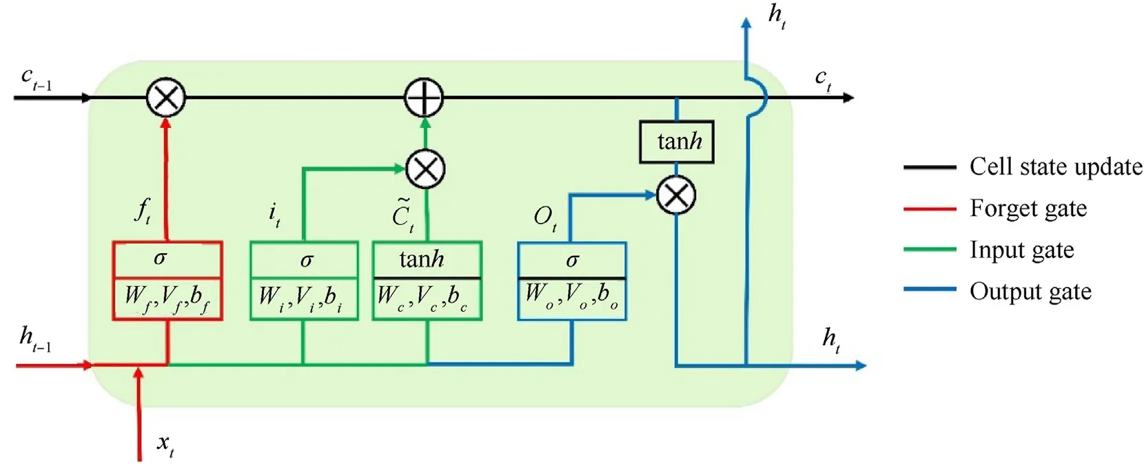
Fig.1. A typical LSTM memory cell.
where σ andtanhrepresent the sigmoid activation function and the hyperbolic tangent activation function,respectively.Wα,Vαandbα (α = {f,i,o,c}) denote the weight matrices which are learned during training process corresponding to different gates(e.g.,forget gate, input gate or output gate). ~ctis a vector of intermediate candidate values created in the input gate shown in Fig.1, and Θ means the Hadamard product (e.g. the element-wise product).
2.2. Dynamic response prediction model with potential LSTM-based architecture
2.2.1. One-layered/stacked LSTM model
LSTM has been proven to have powerful modeling and prediction capabilities when processing data with the features of oscillation and nonlinearity [35], such as a series of electrocardiogram signals. With a more complex and deeper network structure, the stacked LSTM network mainly composed of stacked LSTM layers and fully connected layers has great potential to effectively and accurately model and predict the structural dynamic responses.Fig.2 depicts the overall architecture of the stacked LSTM network,including stacked inputs and outputs. To better illustrate this kind of network, both input and output are assumed to have only one feature, and the number of hidden layers containing LSTM cells is equal to 2.By contrast,One-layered LSTM model contains only one LSTM hidden layer.As shown in Fig.2,while the output of the LSTM hidden layer is propagated forward through time,it is also utilized as one of the inputs of the next LSTM hidden layer. The last two layers are fully connected layers,connecting the LSTM layers to the output layer to build the required number of output features.
As shown in Fig. 2, the stacked LSTM network is divided into 6 parts: an input layer, a reshaping and rescaling layer, the dropout layer, two LSTM layers, two fully connected layers, and an output layer. Each layer is described separately as follows.

Fig. 2. The architecture of stacked LSTM for modeling and predicting (c(β)a and h(β)a represent the cell state and the output of the α cell in the β layer).
(1) The input layer.The input of the network is denoted asX={x1,x2,…,xt,…,xn}T∈Rn×p, wherepandnrepresent the number of input features and time steps, respectively.Xis the matrix with rows standing for time steps and columns for monitoring response features (e.g., load and acceleration).
(2) The reshaping and rescaling layer.It should be noted that the input data fed into the LSTM layers must specify the shape,that is,the input to LSTM layers must be three-dimensional.This expected structure of input data can be formatted as a three-dimensional array[m,n,p],wherem,nandprepresent the number of samples, time step, and input features,respectively. However, the input variables have different units that in turn increases the difficulty of modeling sequences.In this paper,standardization is used to preprocess the input data,which is expected to make the learned model obtain more accurate predictions.
(3) LSTM layers.As illustrated in Fig.2,stacked LSTM network is a deep architecture that consists of more than one LSTM layer,and each LSTM layer is connected to each other by the dropout layer.Here,the number of LSTM layers is assumed to be equal to 2 for better illustration.Firstly,the data processed after the reshaping and rescaling layer is fed into the first LSTM layer with many LSTM cells.Each cell is connected with its two neighbors via {t-1,t,t+1} and would have its own output“h"and cell state“c".The output“h"will then be sent to the next LSTM layer. It should be noted that the hyperparameters (e.g., the number of neurons, the number of hidden layers,etc.)in LSTM layers are selected empirically or using the patterns that have been quoted in research papers.
(4) Dropout layers.A dropout layer is added after the first LSTM layer. When the input vector passes through the dropout layer,part of the information is discarded,which can reduce redundancy and increase the orthogonality between each feature [36]. The dropout layer can reduce overfitting and improve the robustness and generalization ability of the model [37].
(5) Fully connected layers.The last two layers of the network are fully connected layers. Through these layers, the output vectors after going through LSTM layers and dropout layers can be converted into the desired format, which is to build the required number of output features,and passed into the target output layer.
(6) The output layer. The output of the network is denoted asY= {y1,y2,…,yt,…,yn}T∈Rn×q, whereqrepresents the number of output features.Yis the matrix with rows standing for time steps and columns for features (e.g., velocity).
2.2.2. Attention-LSTM model
Motivated by several successful applications of the attention mechanism in natural language processing, the attention mechanism was introduced into LSTM and then a dynamic response prediction model based on Attention-LSTM was proposed. Here,the main purpose of using the attention mechanism is to update the input of the model by assigning weights to input information.This new input can pay more attention to the specific input feature,effectively extracting key features and ignoring redundant features.The proposed Attention-LSTM model for dynamic response prediction is illustrated in Fig. 3. It can be noticed that unlike the stacked LSTM model,the Attention-LSTM model adds an attention layer before the LSTM layer to highlight the key information of the input features.
2.3. Damage indicator extraction
The blast-induced vibration analysis is widely used for structural safety control under blasting, and the peak particle velocity(PPV) is an important and effective indicator used to describe the damage status of a structure [38,39]. Recent research on blastinduced vibration effects indicates that the single vibration intensity factor of PPV cannot fully reflect the structural dynamic responses and the damage status of the structure is also closely related to the vibration frequency [40]. Therefore, it is a feasible approach to extract the damage indicators (i.e., PPV and domain frequency) from the vibration response histories, where the domain frequency denotes the frequency corresponding to the peak of the frequency spectrum power spectral density curve from spectral analysis.
However, the monitoring data of the dynamic SHM system is usually not a specific frequency value, and the method of discrete Fourier transform cannot process the unevenly sampled data. This problem also exists in the structural dynamic responses through FE generation. In this study, the frequency is estimated using the Lomb-Scargle Periodogram.Given a time seriesXj,j=1, 2, …,Nat respective observation timestj(not necessary evenly spaced), the first step is to calculate the signal’s meanand variance (σ2)within the window of size N.Rather than just taking dot products ofthe data with sine and cosine waveforms directly,Scargle modified the standard periodogram formula to first find a time delay τ such that this pair of sinusoids would be mutually orthogonal at sample timestj,and also adjusted for the potential unequal powers of these two basic functions, to obtain a better estimate of the power at a frequency [41]. The time delay τ is defined by the formula
The periodogram at frequency ω is then estimated as
wherePN(ω) is the normalized periodogram (spectral power as function of ω).
Different from the traditional discrete Fourier transform, the spectral power in Lomb-Scargle Periodogram is calculated for every desired frequency, which does not need to be an integral multiple of the inverse of the time window. Therefore, the Lomb-Scargle Periodogram can reveal if a signal’s power is concentrated around a specified frequency value, rather than only at fixed harmonics as the discrete Fourier transform.
2.4. Damage assessment model
The third task of the proposed SHM framework is to establish the correlation between evaluation indicators and damage status.Obviously, this is a classification task in supervised learning. Here,an MLP is defined and configured for multi-label classification.MLP is an artificial neural network with a forwarding structure.Besides the input layer and the output layer, it generally contains one or more hidden layers. Each hidden layer has a certain number of interconnected components called neurons or nodes, which are connected to each other through a certain weight function.
It should be noted that the number of variables in the input layer and nodes in the output layer is determined. Specifically, the number of input variables is equal to the feature dimension of the extracted samples, and the number of output nodes is set to the number of dam damage levels.The remaining hyper-parameters of the model,such as the number of hidden layers,and the selection of the activation function,are optimized by the K-fold cross-validation method. The steps of hyper-parameter optimization and optimal model evaluation implementing K-fold cross-validation are listed as follows:
Step 1:Split the entire classification data set into the training set and the test set according to the ratio of 9:1 as shown in Fig.4,and determine the hyper-parameters to be optimized, and define the search space.
Step 2:Choose a combination of hyper-parameters and build the model.
Step 3: In K-fold cross-validation, the training set is randomly divided intoksubsets. In theseksubsets, one single subset is retained and used as test data for model performance evaluation,and the remaining subsets are used as training data for model training,as shown in Fig. 4.

Fig. 4. Examples of ways to partition a dataset in K-fold cross-validation.
Step 4: Train and test the built model forktimes until all the subsets are given an opportunity to be used as the test data.
Step 5: Repeat Step 2- Step 4 until all hyper-parameter combinations are traversed.
Step 6:Select the model with the best performance in the crossvalidation process, and evaluate the prediction performance and generalization ability of the selected model on the test set.
2.5. Model performance evaluation
2.5.1. Evaluation metrics for dynamic response prediction model
The first two tasks of the deep learning based SHM framework involve prediction accuracy of the dynamic response histories, as well as the extracted damage indicators from them. The development of the dynamic response prediction model is a process of regression predictive modeling.In addition,peak vibration velocity and domain frequency should also be utilized separately as the evaluation metrics for the dynamic response prediction model since these two parameters are two important indicators for the assessment of the dam damage level. In this study, the root mean squared error(RMSE)is utilized to evaluate the performance of the proposed dynamic response prediction model, and the mean absolute error (MAE) and the absolute error ratio (AER) are used to evaluate the prediction accuracy of damage indicators (i.e., peak vibration velocity and domain frequency).MAE,AER,andRMSEare calculated according to Eq. (4), Eq. (5) and Eq. (6), respectively.
wheremis the number of samples, ^ypeakandypeakare the modelpredicted and experimental peak vibration velocity (or domain frequency). And in Eq. (6),nis the number of values,ypandyiare the model-predicted and experimental feature results in response histories.
2.5.2. Evaluation metrics for damage classification model
The last task of the proposed SHM framework involves the classification problem. TheAverage Accuracy[42], which is one of the most frequently used measures in multi-class classification for many classesCi, will be used to evaluate the performance of the damage assessment model.Average Accuracyreturns an overall measure of how much the model is correctly predicting on the entire data set, which can be calculated according to Eq. (7).
wherelrefers to the number of target classesCi, andTPiare true positive counts forCi.Similarly,FPi,FNi,andTNiare counts of false positive, false negative and true negative, respectively.Average Accuracycan also be directly computed from the confusion matrix.The confusion matrix is al×lmatrix,each row of which represents the instances in an actual class while each column represents the instances in a predicted class. It can be found that the correctly classified elements are located along the upper-left to lower-right diagonal of the confusion matrix. Therefore,Average Accuracyis the sum of the diagonal elements divided by the sum of the total matrix elements.
3. LSTM-based blast response prediction for SDOF system
3.1. Data generation by SDOF system
The dynamic motion of concrete gravity dams subjected to blast loads can be simplified as an SDOF system by assuming one ordinate since usually the transverse displacement of the dam crest is another important damage indicator in dam safety control. The system can be described by a spring-mass system in which the equivalent dam mass,equivalent blast load and resistance load are incorporated. The idealized SDOF system is described by the following equation of motion [43,44]:
wherex(t)and ¨x(t)represent the displacement and acceleration of the dam, respectively.R(x) is the resistance as a function of the displacement, andF(t) is the loading as a function of time.Mrepresents the mass of the dam.KLMandcrepresent the load mass factor and the equivalent damping coefficient, respectively.
As part of the analytical study,the blast response of the test dam was predicted using a dynamic nonlinear SDOF analysis. The resistanceR(x)is a polyline,where the resistance linearly increases with the displacementR(x)=kxbefore the plastic damage occurs.Once the displacement exceeds the critical value (x>xc), the resistance remains unchangedR(x) =kxc. It is also noted that the damping effects are neglected in the present SDOF model because the duration of the blast event is very small compared to the natural time period of the dam [6]. Then, the equation of motion and the initial condition can be described as Eq. (9) and Eq. (10), respectively [45,46]. In this subsection, the blast load is idealized as the triangle shape, and the main load parameters (i.e., the peak reflected pressure and duration) can be generalized by Eq. (11)[43,44].
In this subsection, data generated through the SDOF system considered the variability of blast load (i.e., charge weight and standoff distance) and structural resistance. Based on the given ranges of charge weightWand standoff distanceR, the resulting scaled distance can be calculated byZ=R/W1/3,as well as the peak reflected pressurePrand durationtd. As shown in Table 1, all the related parameters of the SDOF system are listed for the dynamic response solution.The sampling frequency and data length are set to 2000 Hz and 200 ms, respectively. At first, a total of 2000 samples(i.e.,802000 data points)are generated using the Runge-Kutta Method numerical integration method.

Table 1Related parameters of the SDOF system for dynamic response solution.
For real-world problems, noise from the sensor itself, ambient vibration, or even temperature variations is usually inevitable during the data-collection process. In this study, white noise technique is used to simulate the monitoring noise in the original monitoring acceleration histories with a zero mean but a non-zero standard deviation.Five noise levels(i.e.,1%, 2%,5%,10%, and 30%)were considered to simulate practical situations, and each noise signal was obtained by multiplying the noise level with standard deviation of each vibration signal. Therefore, another 10000 samples (i.e., 4010000 data points) with five different noise levels are generated for noisy effect analysis.
3.2. LSTM-based models for dynamic response prediction
In this subsection, LSTM-based models are used to predict the response of the nonlinear SDOF system.The performances of these three deep learning models with respect to non-noisecontaminated input and output signals are compared and discussed.In general,without prior knowledge of the SDOF structural model, physical understanding of the problem suggests that the maximum vibration velocity and displacement of the structure under a given pulse loading are used to compare with the critical characteristic associated with a given damage level. Thus, for the SDOF system herein,the input-output relationship is considered to predict the velocity and displacement with acceleration and excitation. After training the LSTM-based models with non-noisecontaminated data, each model was trained again using noisy input and noisy output data. Five noise levels (i.e.,1%, 2%, 5%,10%and 30%) are added to the original signals to investigate the robustness of these LSTM-based models against noisy data.
A number of 2000 samples are generated, and each sample is composed of load and acceleration as input and velocity anddisplacement as output. All of the samples are split into three subsets with the ratio of 8:1:1,including the training set with 1600 samples, and both validation set and test set with 200 samples. In addition, since the data fed into LSTM layers should be threedimensional and each sample has 401 time steps, the input and output formats are reshaped as [1600,401,2] and [1600,401,2] for training and validation, respectively. In this study, the LSTM cell implemented by the deep learning framework of Keras with Tensor Flow as a backend has been used for the experiments. A server equipped with 4 NVIDIA GP104GL[Tesla P4]Graphics Cards is used to train and evaluate the models.
Three types of models were verified on the SDOF generated data,namely a One-layered LSTM model,a Stacked LSTM model,and an Attention-LSTM model.For these LSTM-based models,some hyperparameters, such as batch size, epoch number, number of hidden LSTM layers,and number of LSTM cells per hidden layer,affect the performance of the model.Typically,the considered range for each tuning hyper-parameter is selected empirically or using grid searching method and the patterns that have been quoted in research papers. For the number of hidden LSTM layers, {1—5} are examined, and the stacked LSTM containing 2 LSTM layers is capable of predicting future sequence and outperforms any other configuration. Additionally, the number of LSTM cells per hidden layer is considered to be set to 100 as described and implemented in Ref. [46]. A batch size of 1000 and an epoch of 500 are used to train the model. Noted that both the Stacked LSTM model and the Attention-LSTM model have the same LSTM architecture for comparison purpose,except that the Attention-LSTM model introduces an attention layer before LSTM layers.
During the training process, the rectified linear unit (Relu) is used as the activation function. The mean squared error (MSE),which is one of the commonly used loss functions for sequence prediction tasks, is utilized as the loss function for learning the parameters.To accelerate the convergence of training these LSTMbased models, Adam (Adaptive Momentum Estimation) optimizer is selected to minimize the loss function for each batch with a learning rate of 0.001 and a decay rate of 0.0001.
3.3. Evaluation on LSTM-based models for dynamic response prediction
Fig. 5 illustrates the training and validation loss curves of the three models for the non-noise-contaminated data. The training phase consists of 500 epochs to ensure the convergence of the loss function. In fact, the training and validation losses of the three models continue to decrease as the epoch increases,and the curves are starting to be stable from 100 epochs. It is shown that all the models can lead to very small training loss values (approximately 0.002) and validation loss values (approximately 0.01), indicating their excellent performances to predict the structural dynamic responses. After the training and validation of these LSTM-based models, the test data are fed into the models, including 200 samples, and test the reliability of these models for the data that independent on the training set.
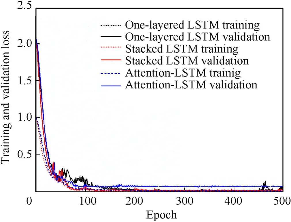
Fig. 5. The training and validation loss of three LSTM-based networks.
For example, the prediction performance of Stacked LSTM model based on a sample data is illustrated in Fig. 6. It is obvious that the Stacked LSTM model is capable of depicturing the general rule of the structural dynamic responses of nonlinear SDOF system with a high accuracy (the black solid line and the blue dash line),even though there exist some gaps at the peaks. That means the Stacked LSTM model can solve the integral problems,i.e.,predicting the velocity and displacement histories with acceleration. Moreover,this study also considers the inevitable noise during the SHM.As show in Fig.6,when 10%noise is added to the monitoring signals as an example (the red solid line), the prediction precision of velocity and displacement both will be relatively attenuated, especially near the peak values(the pink dash line).It can be concluded that the Stacked LSTM has a strong ability to resist noise interference.

Fig. 6. Prediction performance of Stacked LSTM model based on a sample data: (a) Prediction of velocity history; (b) Prediction of displacement history.
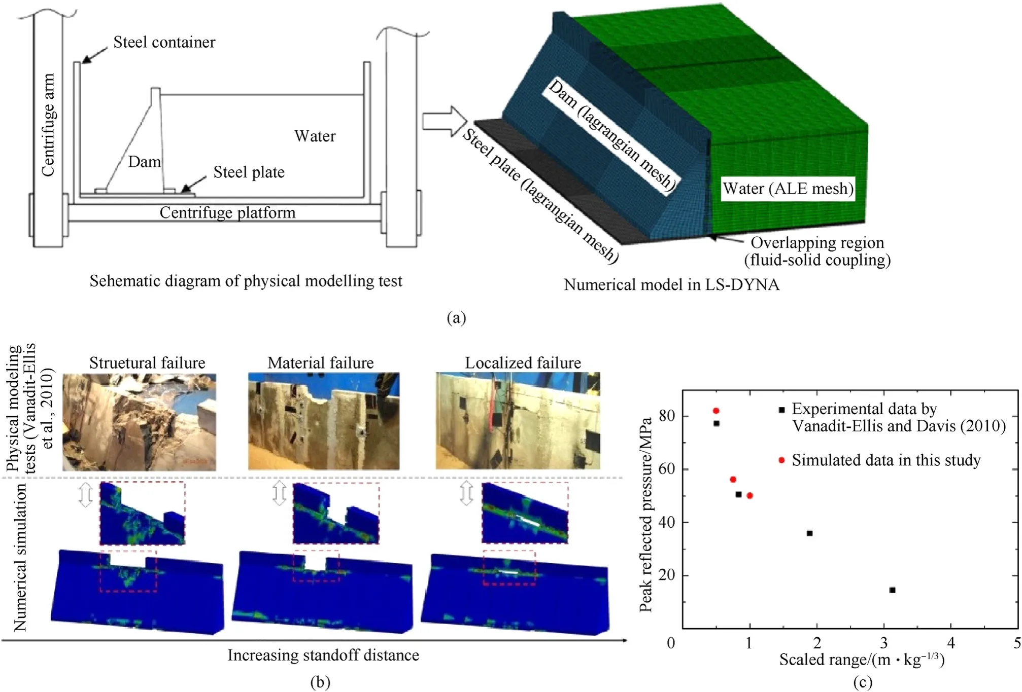
Fig.7. Numerical method verification:(a)Numerical model in LS-DYNA;(b)Comparison of the failure modes;(c)Comparison of the peak reflected pressures on the front face of the model.
To further evaluate the prediction performance of each model and the adaptability to different noise levels,the averageRMSEsof using monitoring acceleration and excitation to predict the velocity and displacement are listed in Table 2.When the input monitoring histories are contaminated by different noise levels, theRMSEsof velocity given in the third column represent the prediction errors between the model-predicted and integral velocity histories with the noise-contaminated acceleration histories.While,theRMSEsof velocity given in the fifth column represent the prediction errors between model-predicted velocity with noise-contaminated acceleration and integral velocity with non-noise acceleration,which is defined as the results with respect to ideal in this study.The same definition is also used in the evaluation of displacement prediction in fourth and sixth columns.In general,theRMSEincreases with the noise level,and all LSTM-based networks achieve good estimations with a relatively lowerRMSE, though they are trained with the noise-contaminated signals. Moreover, these three LSTM-based models show better prediction performance to the velocity histories (in the magnitude of 10-4m/s) than those to displacement histories(in the magnitude of 10-2m).As shown in Fig.6 and Table 2, the higher prediction error of displacement histories may be caused by the error accumulation of the time history analysis.In practice, the signal noise is inevitable for the operation environment of the structures and monitoring equipment.Thus,it may be more reasonable to evaluate the structure health status with the velocity indicator rather than the displacement indicator during the SHM analysis under dynamic loads.
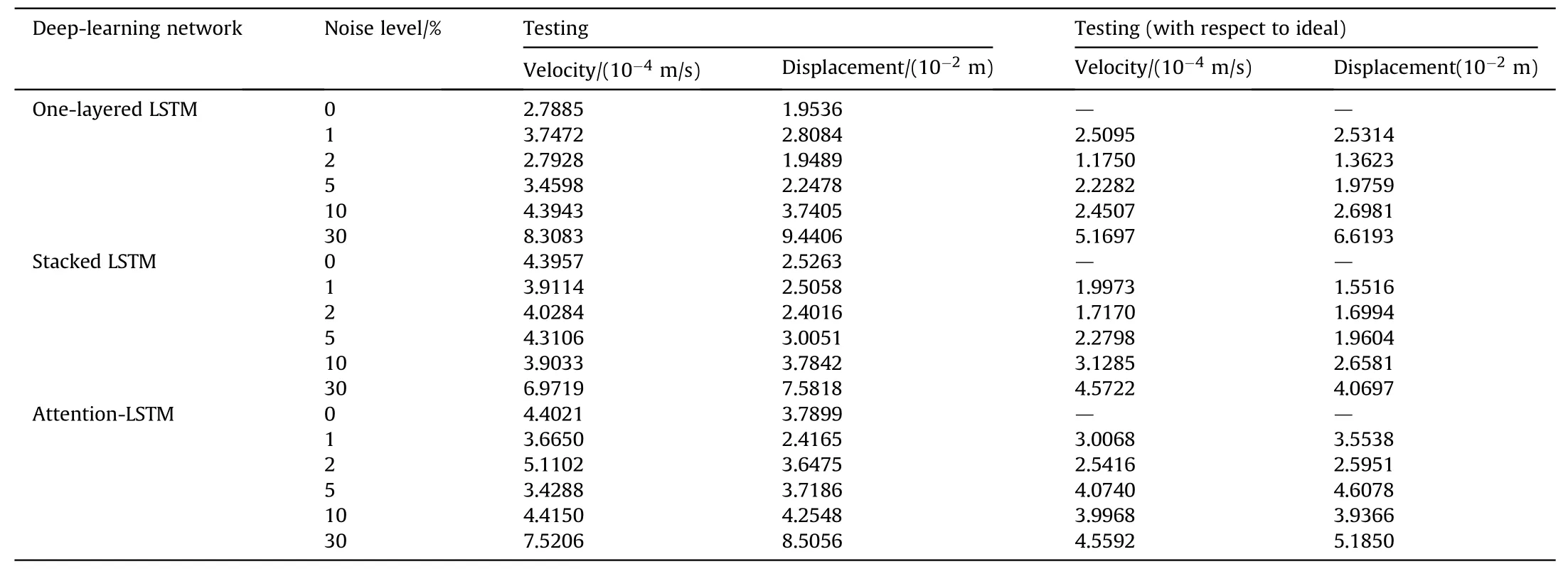
Table 2Average RMSE for three deep-learning models using different noise-contaminated signals.
For these LSTM-based models, their prediction accuracies against to different noise levels are similar, and among them the Stacked LSTM performs relatively best to the ideal cases (i.e., 0%noise).For example,under the 1%noise level,theRMSEof predicted velocity histories for Stacked LSTM model is only 1˙9973×10-4m/s with respected to the ideal target, while 2˙5095×10-4m/sRMSEfor One-layered LSTM model and 3˙0068×10-4m/sRMSEfor Attention-LSTM model. In addition, the prediction accuracy of these models with respect to the ideal target always higher than those with respect to the noisy target.That means the above LSTMbased models can catch the general rule of structural dynamic response, eliminating the effect of monitoring noise and receiving an acceptable prediction accuracy.
4. Dynamic response estimation on concrete gravity dam under explosions
4.1. Verification of the numerical method
Fig. 7(a) shows the physical modeling tests conducted by Vanadit-Ellis and Davis [3], which are used to verify the fully coupled numerical model and the input parameters on LS-DYNA platform, whose origins and core-competency lie in highly nonlinear transient dynamic finite element analysis (FEA) using explicit time integration. The fluid-structure interaction herein is solved by Arbitrary Lagrangian-Eulerian (ALE) method [5—7]. The Continuous Smooth Cap model (CSC model) is employed to simulate the nonlinear dynamic behaviors of concrete and its model parameters are discussed carefully in Refs.[6,7].Also,the material models and input parameters of TNT explosive and water are determined according to previous studies [6,7]. In this subsection,the transmission boundary conditions are adopted along the truncated boundary, and the surface-to-surface contact is used to model the nonlinear contact behavior between dam sections with a friction coefficient of 0.80. As for the explosive source, The charge weight and the detonation depth remain 8 g TNT equivalent and 0.025 m below the water surface,but the standoff distance varies to be 0.10 m, 0.15 m, and 0.20 m.
As a result, Fig. 7(b) compares the failure patterns from numerical simulation and physical modeling tests. It is obvious that the present numerical method can capture the general failure patterns of dams subjected to underwater explosions. The blastinduced failure of concrete gravity dams were concluded into three types, i.e., material failure, localized failure, and structural failure. Moreover, the recorded peak reflected pressures in both numerical simulations and physical modeling tests share the similar trend along with the scaled distance. More details of the coupled numerical method can be seen in our previous works[6,7].In addition,Vanadit-Ellis and Davis(2010)also recorded the shock waves on the front face of the model and gave the peak reflected pressures at different scaled distances in the literature.The records at the depth of 0.127 m on the upstream dam surface is used to verified the numerical results. As shown in Fig. 7(c), the peak reflected pressures from numerical simulations located near the trend line of the experimental data, further indicating the validation of the method in this study. Mention that the PETN based explosives was used in the physical model tests and all the data in Fig. 7(c) are transformed and compared in term of equivalent TNT charge.
4.2. EF dataset generation
A concrete gravity dam located in Northeast China is used as the case structure to evaluate the proposed method,which had served for 66 years and was demolished by blasting in 2018 as shown in Fig. 8(a). The dam section nearest to the explosive source is analyzed herein since it is the most serious damaged partition when an underwater explosion occurs [7]. The FE model was constructed according to the verified numerical method. As shown in Fig. 8(b), the overall elevation above ground level is 89.5 m. The transmission boundary and the symmetrical boundaries are implemented to simplify the numerical model. The mesh sizes of 100 mm and 200 mm are to discretize the explosive and dam head,and the mesh refinement method is employed for the areas near the explosive. For simplification, the material partition is not considered in this study, and the property of dam concrete were generated as density 2400 kg/m3, elastic modulus 24 GPa, and Poison’s ratio 0.17 [7]. Also, the initial stress field induced by the gravity, uplift pressure, and hydrostatic pressure is considered in this study before explosions,as shown in Fig.9(a).More details are introduced in our previous work[7].

Fig. 8. Establishing of FE model: (a) The old dam to be demolished; (b) Configuration of the FE model.
Before blast-resistance analysis, spectral analysis is conducted under the empty reservoir condition. Table 3 lists the first five natural frequencies,comparing with the results of the field test and the analysis by Chi et al. [47]. As a result, the calculated values in this study approximate to those analyzed by Chi et al. [47]. Moreover,the basis frequency is about 17%lower than the experimental value. That is to say, the dynamic stiffness is relatively lower than that of practical structure. Maybe, the estimation of the dam concrete is too low or the range of the low-grade concrete is not considered in the FE model construction.

Table 3Comparison of the spectral analysis results.
Then, various explosion scenarios are simulated considering standoff distance (5 m,10 m,15 m, 20 m, 25 m), detonation depth(10 m,22 m,32 m,45 m,60 m)and charge weight(100 kg,200 kg,400 kg,600 kg,800 kg,1000 kg).During operation,the water level usually changes between normal and dead water levels and thus the effect of variation in water level is considered as 263.5 m,252 m and 242.5 m.Moreover,it is surveyed that the concrete strength of the dam grows over time with a logarithmic curve [48,49], the tested concrete strength is taken as 15 MPa,20 MPa,or 25 MPa here according to the findings. For all the cases, as shown in Fig. 9(a), a set of accelerometers (i.e., Ps1, Ps2, …, and Ps5) are installed on different locations to record acceleration measurements and a pressure sensor at the upstream surface (i.e., Ac1) is also used to record the load.Each explosion scenario was calculated for 150 ms,which was long enough for all explosion scenarios to reach the steady stage of dam damage. At last, as illustrated in Fig. 9(b), the histories of load and dam dynamic responses(including horizontal and vertical acceleration, velocity, and displacement) installed to the specific locations are extracted from the simulated results, as well as the figures of the final dam damage status.Fig.9(a)gives the definition of crack penetration ratio, which is the ratio of penetration depth (lp) to cross-sectional length (lcs), i.e., Pr= lp/lcs. The higher the penetration ratio for a crack is,more likely a dam-break flood will be to form.
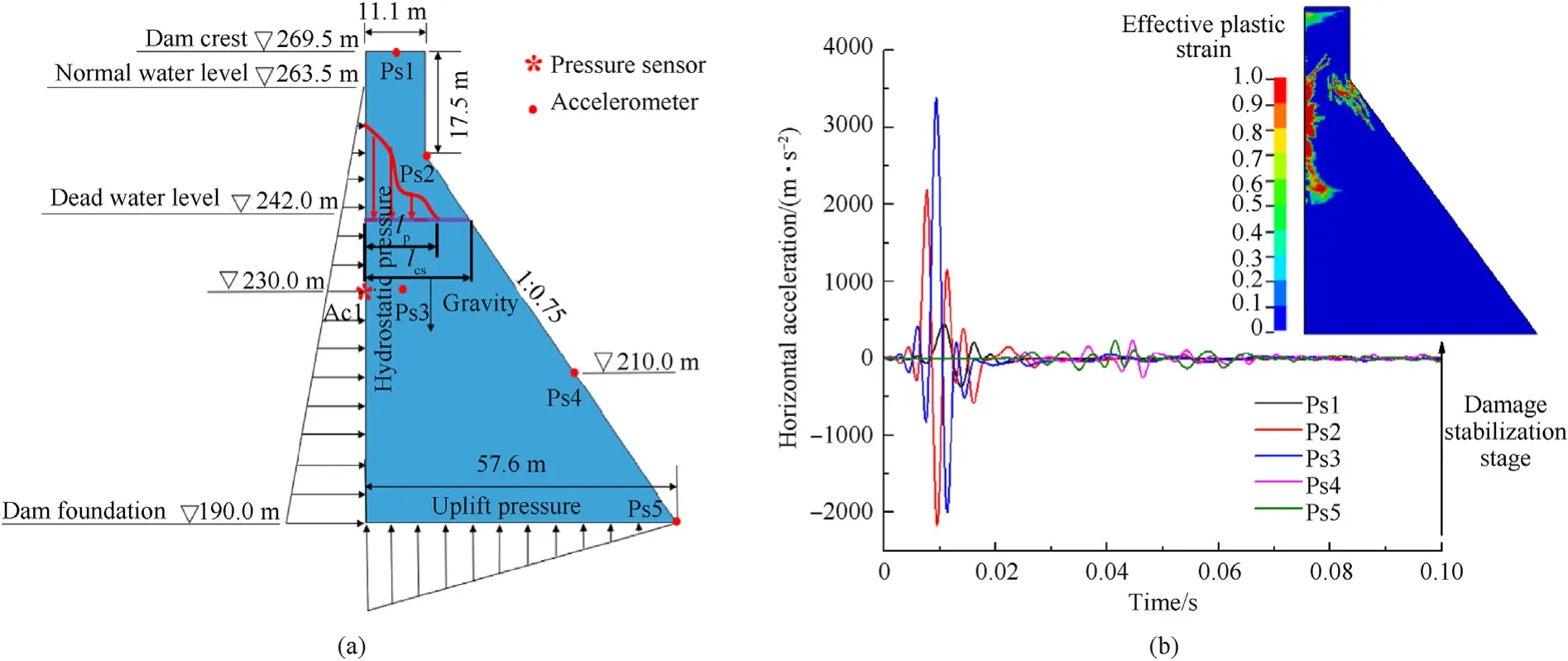
Fig. 9. Monitoring data extraction: (a) Dam monitoring scheme and definition of the crack penetration ratio; (b) Data acquisition from numerical results.
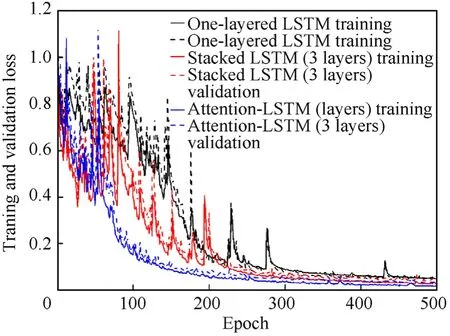
Fig. 10. The training and validation loss of three LSTM-based models against the number of epochs.
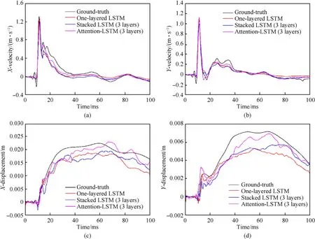
Fig.11. Comparison of predicted and numerical results for a single sample(water level(W)of 263.5 m;standoff distance(R)of 10 m;detonation depth(D)of 10 m;charge weight(Q) of 400 kg; concrete strength (fc) of 20 MPa).
According to the blast-resistance criterion of concrete gravity dam proposed by Wang and Zhang [5], the dam damage was divided into four levels,i.e.,no damage(remaining in elastic state),slight damage(the penetration degree of cracks on dam less than 1/3), moderate damage (the penetration degree of cracks on dam exceeding 1/3 but less than 2/3), and severe damage (the penetration degree of cracks on dam exceeding 2/3). It should be mentioned that these definitions of present damage levels are subjective. Similar damage categories can also be found in literatures[6,7,28].
4.3. Dam health diagnosis with deep learning network
4.3.1. Evaluation on the dam dynamic response analysis of proposed SHM framework
The LSTM-based models are further verified using numerical simulation data. Load on the upstream surface of the dam and accelerations in thexandydirections are used as inputs, while the displacements and velocities in thexandydirections are used as outputs. The time history of load, acceleration, displacement, and velocity recorded at each measuring point in each case is taken as a sample, and therefore a total of 900 samples (180 cases and 5 monitoring points in each case) from numerical simulation can be obtained. The data set is still split into three subsets according to the ratio of 8:1:1,including 720 samples for training,90 samples for validation,and 90 samples for testing.The input and output sizes of the training dataset are[3,720,1000]and[4,720,1000],respectively.Obviously,the relationship between the input and the output from the numerical simulation is more complicated than that is from a single degree of freedom.Therefore,the prediction model based on LSTM has a more complex structure.
The same LSTM cell, loss function and activation function as in SDOF are adopted here except for the different number of LSTM layers.Fig.10 shows the loss curves generated by the three models using numerical simulation data for training and validation.Before 300 epochs,there still exists some large loss values for these LSTMbased models,and the loss curves oscillate up and down.After 300 epochs, the loss value gradually stabilizes. It can be seen from Fig.10 that the loss of the One-layered LSTM model has the slowest convergence, and the loss curve in the early stage oscillates frequently and is unstable,in contrast to the Attention-LSTM model that has 3 LSTM layers with the fastest convergence and the smallest amplitude oscillation. The Attention-LSTM model (3 layers) performs relatively better than the One-layered LSTM model and the Stacked LSTM model(3 layers)with a much smaller training loss value (0.0006) and a validation loss value (0.012).
By feeding the test data into these three trained models, the predicted responses of different models can be obtained as illustrated in Fig. 11 in comparison with the ground-truth for an example. It is shown that all these three trained models are generally capable of picturing the common trends of dam dynamic responses under explosions, especially for the velocities in both two directions. Moreover, these trained LSTM-based models can well describe the peak vibration velocity of dam dynamic responses under explosions, and the main differences of prediction performance lie in the displacement responses. Among all the trained LSTM-based models, the Attention-LSTM model (3 layers) shows the best prediction performance,both in velocity and displacement responses. The prediction performance of Attention-LSTM is further illustrated in Fig.12 for different explosion scenarios.It can be concluded that the Attention-LSTM is able to adapt different explosion parameters with a high prediction performance of velocity and displacement. This conclusion is consistent with that in SDOF analysis, and the reason is explained by the error accumulation of the predicted dynamic response.
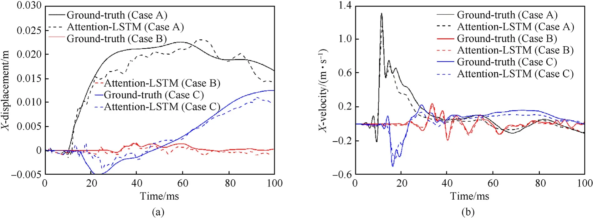
Fig.12. Performance of Attention-LSTM model for different explosion scenarios at Ps1(Case A:W=263.5 m,R=10 m,D=10 m,Q=400 kg and fc=20 MPa;Case B:W=242.5 m,R = 25 m, D = 60 m, Q = 400 kg and fc = 20 MPa; Case C: W = 252 m, R = 15 m, D = 22 m, Q = 600 kg and fc = 25 MPa).
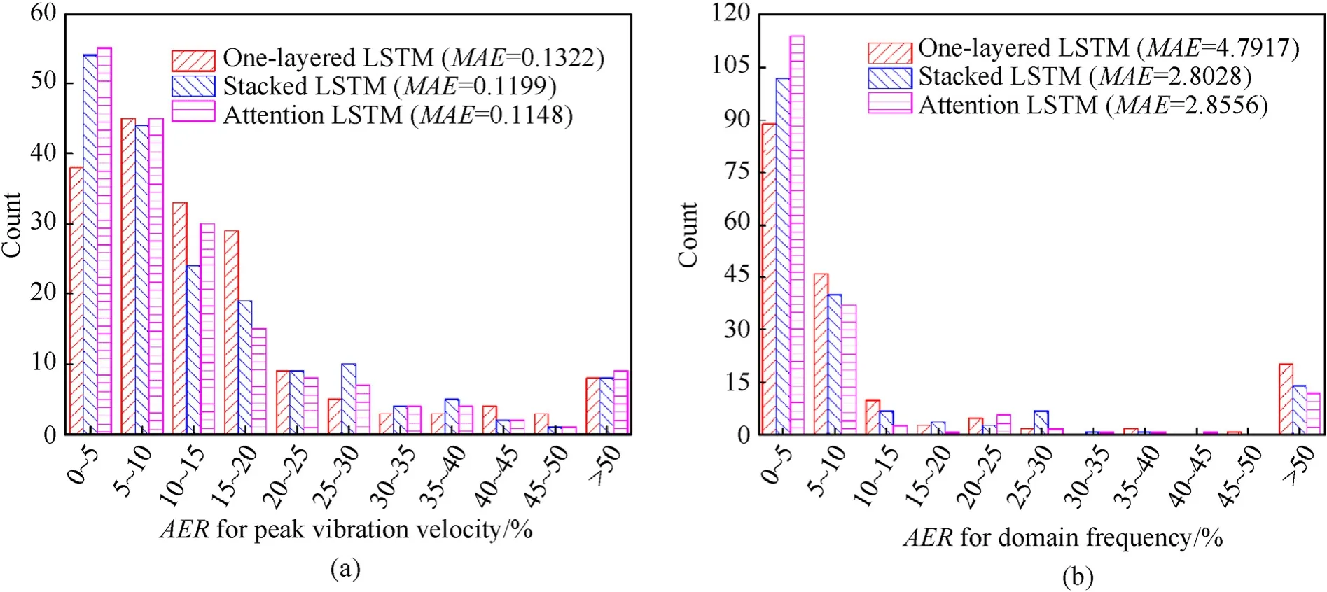
Fig.13. Test performance of three LSTM-based models: (a) Peak vibration velocity; (b) Domain frequency.
Based on the conclusion above,this study suggests to extract the main damage indicators from velocity histories to assess the structural damage status.As has been done in many literatures and engineering [6,40], the peak vibration velocity and the corresponding domain frequency are widely used to control the blasting and maintain the structural safety.The peak vibration velocity and domain frequency in thexandydirections of each measuring point are extracted from the time-histories of velocity responses.So that,the peak vibration velocity and domain frequency are also compared between predicted and simulated velocity histories to assess the performances of these three LSTM-based networks according to Eq. (5).
As shown in Fig. 13, the absolute error ratio (AER) is used to assess the prediction performance,as well as theMAE.It is obvious that the One-layered LSTM network shows the highest prediction errors both in terms of peak vibration velocity and domain frequency. Although theMAEs of Stacked LSTM and Attention LSTM networks are quite similar with respect to peak vibration velocity and domain frequency, their error distribution in terms ofAERshows somewhat differences. The Attention-based model with relatively smallerAERvalues performs better than the Stacked LSTM network.As forAERof peak vibration velocity less than 15%,the count for Attention LSTM network reaches 130(about 72.22%),while that for Stacked LSTM network reaches 122 (about 67.78%).More obviously, as forAERof domain frequency less than 10%, the count for Attention LSTM network reaches 151 (about 83.89%),while that for Stacked LSTM network reaches 142 (about 78.89%).
Clearly the Attention-based model with relatively small MAE values performs better than both the One-layered LSTM model and the Stacked LSTM model.However,another finding discovered here is the fact that the prediction performance of the Attention-LSTM model is not as good as expected, and the Stacked-LSTM does not significantly outperform the One-layered LSTM in the context of SDOF.The possible reason is that SDOF is a single degree of freedom system,while the numerical simulation is a high degree of freedom system.In SDOF,the relationship between input and output is less complicated compared to numerical simulation, and the application of deeper and more complex models will not improve the predictive ability due to the possibility of over-fitting,resulting in a poor generalization ability. In numerical simulation, there is a complex and non-linear relationship between input and output,and the Attention-LSTM model shows outstanding prediction effects.It could be the reason that for more input and output features,as well as long-term time series prediction, the Attention-LSTM model has a deeper network that can dig out the complex correspondence between the input and the output. Additionally, the Attention-LSTM model brings advantages of selecting the important and relevant information, thereby improving the prediction accuracy.
4.3.2. Evaluation on the damage assessment analysis of proposed SHM framework
In this study,peak vibration velocity and domain frequency are introduced to evaluate the damage level of the dam. Taking the peak vibration velocity and domain frequency in thexandydirections of each measuring point as input,and three damage levels as output,a total of 180 cases can be obtained.The data set are still used in the regression model.Among them,162 classification cases are utilized as the training set for K-fold cross-validation to find the optimal network structure. In addition,18 classification cases are adopted as the test set for the performance evaluation of the trained optimal model.
The 10-fold cross-validation method(K=10)is used to evaluate different hyper-parameter combinations of hidden layers and then determine the final structure of the model. Then, different hyperparameter combinations are tested to decide which one is the best configuration as the result.For example,the number of hidden layers ranges from 1 to 10,while the number of epochs is examined from {500, 1000, 2000, 5000, 10000}. The optional activation functions are tanh, relu and sigmoid. The batch-size is selected from {4, 8, 16, 32, 64, 128, 256, 512, 1024}. In the 10-fold crossvalidation, the training set is divided into 10 parts, with 1 part randomly selected as the verification,and others used for training.After training,the structure of the optimal model that produces the best classification accuracy is given in Table 4. It should be noted that the output layer of the model is fixed to achieve a ternary classification. 3 nodes and the “softmax” activation function are required in the end to predict which damage level that a given observation feature set will produce.The number of nodes in each hidden layer is set to 10.

Table 4The parameters used in the damage assessment model.
Fig.14 shows the confusion matrix generated from the classification results using the trained optimal model with the test set.Thenumbers in Fig.14 represent the statistical results of the groundtruth and predictions for the dam damage classification based on the test set of 18 cases. For example, the number “2” in the upper left corner of this figure indicates that there are 2 cases classified as severe damage by the classification model, and these 2 cases actually refer to severe damage as well,which means the proposed classification model can correctly classify these 2 cases as the severe damage. From the confusion matrix, theAverage Accuracyis calculated by 83.33%,and the ratio for underestimation of damage level is only 5.56%.In sum,the peak vibration velocity and domain frequency extracted from predicted velocity histories can well classify the damage status of the dam.So that,the optimized SHM framework proposed in this study can predict the velocity histories with monitoring acceleration data,and further extract the damage indicators from the velocity histories to assess the damage status of the dam experienced underwater explosions.
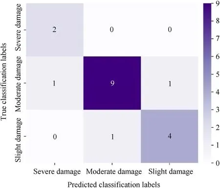
Fig.14. The confusion matrix generated from the classification results.
5. Conclusions
The major challenge of damage diagnosis on the dams experienced explosions lies in the real-time analysis and judgment for emergency decision-making to protect the downstream human lives and property, especially in the condition of unknown explosion source. To address this limitation, this paper introduced a deep-learning based SHM framework, which is one of the major breakthroughs in structural dynamic response analysis, for dam damage diagnosis with monitoring data.
In the deep-learning based SHM framework, the LSTM-based models have been verified to process data and adjust itself to the measuring noise,which holds great potential for real-time dynamic response analysis for both nonlinear SDOF system and FE simulation,with high accuracy,robustness,and computational efficiency.Moreover,all LSTM-based models show better prediction ability to velocity responses than displacement responses. Since the Attention-LSTM network has higher prediction performance for multiple monitoring points,it is suggested to predict the structural dynamic responses in the SHM framework of this study.
As usually done in structural vibration control, peak vibration velocity and domain frequency are suggested to be the indicators of dam damage, which can be easily extracted from the predicted velocity histories via Lomb-Scargle Periodogram method with due consideration of the unevenly sampling in SHM. Furthermore, an MLP network for multi-label classification is used to characterize the unknown relation between damage indicators and damage statuses, and the hyperparameters of the MLP network are optimized by the K-fold cross-validation method. Therefore, the deep learning technique has the ability to discover the abstract features in structural dynamic responses and complex damage status of dams.
Overall, this study proposes a deep-learning based SHM framework for real-time emergency decision-making of the dam once experienced explosions, which is capable of predicting the structural dynamic responses with vibration monitoring data,extracting the damage indicators from the response information,and finally diagnosing the dam damage status. The present work overcomes the challenge of dam damage detection after extreme blast conditions, and proposes a popular SHM framework with deep-learning-based damage identification and classification functions.
Declaration of competing interest
The authors declare that they have no known competing financial interests or personal relationships that could have appeared to influence the work reported in this paper.
Acknowledgements
This work has been supported by a grant from the National Natural Science Foundation of China (Grant No. 52109163 and 51979188).
杂志排行
Defence Technology的其它文章
- A review on lightweight materials for defence applications: Present and future developments
- Study on the prediction and inverse prediction of detonation properties based on deep learning
- Research of detonation products of RDX/Al from the perspective of composition
- Anti-sintering behavior and combustion process of aluminum nano particles coated with PTFE: A molecular dynamics study
- Microstructural image based convolutional neural networks for efficient prediction of full-field stress maps in short fiber polymer composites
- Modeling the blast load induced by a close-in explosion considering cylindrical charge parameters
