Sensitivity analysis of spacecraft in micrometeoroids and orbital debris environment based on panel method

Di-qi Hu,Run-qiang Chi,Yu-yan Liu,Bao-jun Pang

Hypervelocity Impact Research Center,Harbin Institute of Technology,150080,Harbin,China

Keywords:Shielding algorithm Panel method Spacecraft Sensitivity

ABSTRACT To reduce the risk of mission failure caused by the MM/OD impact of the spacecraft,it is necessary to optimize the design of the spacecraft.Spacecraft survivability assessment is the key technology in the optimal design of spacecraft.Spacecraft survivability assessment includes spacecraft impact sensitivity analysis and spacecraft component vulnerability analysis under MM/OD environment.The impact sensitivity refers to the probability of a spacecraft encountering an MM/OD impact while in orbit.Vulnerability refers to the probability that each component of a spacecraft may fail or malfunction when impacted by space debris.Yet this paper mainly analyzes the impact sensitivity and proposes a spacecraft sensitivity assessment method under the MM/OD environment based on a panel method.Under this panel method,a spacecraft geometric model is discretized into small panels,and whether they are impacted by MM/OD or not is determined through the analysis of the shielding or shadowing relationships between panels.The number of impacts on each panel is obtained through calculation,and accordingly the probability of each spacecraft component encountering MM/OD impact can be acquired,thus generating the impact sensibility.This paper extracts data from the NASA's ORDEM2000,the ESA's MASTER8 as well as the SDEEM2015(Space Debris Environmental Engineering Model developed by HIT),and uses the PCHIP(Piecewise Cubic Hermite Interpolating Polynomial)method to interpolate and fit the size-flux relationship of space debris.Compared with linear interpolation and cubic spline interpolation,the fitting results through the method are relatively more accurate.The feasibility of this method is also demonstrated through two actual examples shown in this paper,whose results are close to those from ESABASE,although there are some minor errors mainly due to different debris data input.Through the cross-check by three risk assessment software - BUMPER,MDPANTO and MODAOST - under standard operating conditions,the feasibility of this method is again verified.

1.Introduction

As human further their explorations to the cosmos,decommissioned satellites,mission-related debris,rocket bodies and fragments generated by collisions or explosions of satellites continue to pollute the space environment.The number of objects in Earth orbit officially cataloged by the U.S.SSN has been close to 22,000 by the end of February 2021,yet only less than one fourth are active traceable spacecrafts as shown in Fig.1 [1].In LEO,only particles with diameter larger than 10 cm can be tracked and effectively prevented from damaging spacecrafts through collision avoidance maneuvers.However,smaller objects (0.5-10 cm) pose much more severe threats to other active satellites,because they are numerous,powerful and untraceable.According to the data provided by ESA's Space Debris Office in January 2021,the total mass of all space objects in Earth orbit is more than 9200 tons[2].It is estimated through statistical models that the number of debris objects with the diameter from 1 cm to 10 cm may be around 900,000,whereas the number of debris objects with the diameter from 1 mm to 1 cm is about 128 million.Even more alarmingly,some companies plan to operate satellite constellation in LEO,and with more small satellites launched in the coming decades,the rapid increase of small satellite constellations will worsen the LEO space environment.

Nomenclature

BLEBallistic Limit Equations

EMIErnst Mach Institute

ESAEuropean Space Agency

FEMFinite Element Model

HITHarbin Institute of Technology

LEOLow Earth Orbits

LDEFLong Duration Exposure Facility

MM/OD Micrometeoroids and Orbital Debris

PCHIPPiecewise Cubic Hermite Interpolating Polynomial

PIRATParticle Impact Risk and Vulnerability Analysis Tool

SRLSchafer-Ryan-Lambert

SSNSpace Surveillance Network

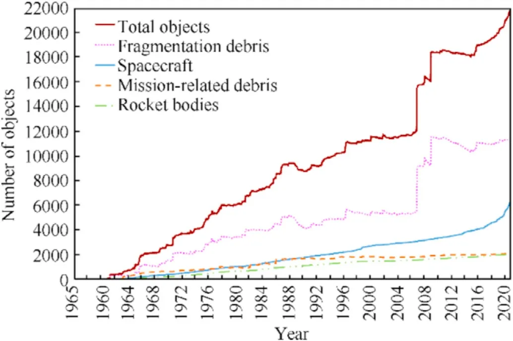
Fig.1.Number of Objects in Earth Orbit cataloged by the U.S.SSN.

To lower the failure risk,the probability of a spacecraft encountering an MM/OD impact during operation in orbit must be properly assessed when designing spacecraft.The impact sensitivity analysis,taking MM/OD as the risk source to investigate the impact probabilities of spacecraft and its internal components,plays a fundamental role in the on-orbit risk assessment of spacecraft.The risk assessment software represented by NASA's BUMPER[3]establishes a FEM of the spacecraft structure,which can be used to analyze the probability of a spacecraft encountering MM/OD impact,but only the outer structure of a spacecraft is analyzed.

At present,the widely used method to analyze the impact sensitivity of spacecraft is the ray-tracing methodology,represented by the ESABASE2/DEBRIS [4] developed by ESA and the SHIELD [5] developed by H.Stokes (QinetiQ) and the University of Southampton,which uses the Monte Carlo method to randomly select the flow direction of debris to generate rays to simulate the impact of space debris on spacecraft.However,in SHIELD,the projectile after first impact on the outer structures will then hit the internal parts with the same mass,speed and direction as those of the first impact.In ESABASE2/DEBRIS,this problem is solved through the use of a debris cloud model.EMI's PIRAT [6] tool replaces internal components by aluminum plates and uses SRL-BLE to solve the shielding problems between components.

In addition,Di-qi HU [7] et al.from Harbin Institute of Technology use a virtual exterior wall method to generate rays to simulate the impact of space debris on spacecraft in all directions.The calculation accuracy of this method reaches the level of ESABASE2/Debris.

Mirko Trisolini [8] et al.proposed a survivability assessment method based on the concept of vulnerable zones.Debris impacts the spacecraft structure to form debris cloud,which will create a conical geometric area.The geometric relationship between the conical geometric area and the internal components is analyzed,and the mutual shielding between internal components is also taken into consideration.And the impact probability of internal components is also calculated.

This paper proposes a novel spacecraft sensitivity assessment method based on the panel method under MM/OD environment.It takes the space debris data from the current space debris environment model as input,analyzes each panel and calculates the impact numbers on each panel,and accordingly the numbers of impacts on each component can be obtained.Based on that,the impact sensitivity of each component is calculated and obtained.

2.Analysis process of impact sensitivity for spacecraft

The analysis process of the impact sensitivity for spacecraft components is shown in Fig.2.To generate the MM/OD flux data of each potential damaging space debris on target orbit,the MM/OD environmental engineering model and the spacecraft motion model are used,then the flux φ with velocity v and size d of each debris can be obtained.At the same time,the outer and inner components of a spacecraft are geometrically modeled,all of which are further divided into panels through finite element grid.The standard k file format[9] is then generated and taken as the input file for the following analysis of the geometric model.In order to get the area of each exposed panel for further calculation,the outer components are selected and analyzed through shielding algorithm.If the panel is shielded,its exposed area is 0.If the panel is not shielded,the area of the exposed panel can be obtained and recorded.With the calculation of the flux φ and the exposed area,the number of impacts on each corresponding panel and thus the component can be obtained.Then according to the probability distribution of impact events,the impact sensitivity of spacecraft components is calculated and acquired.

3.Space debris environment

3.1.Definition of space debris flux

Space debris environment engineering model [10] can help describe the spatial and temporal distribution of the space debris environment through statistical methods.By analysing the movement law of fragments,the flux of debris under different sizes,speeds,and directions can be obtained,which provides necessary input data for subsequent calculation.

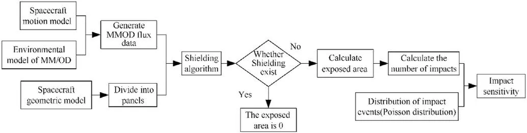
Fig.2.Analysis process of impact sensitivity of spacecraft.

Among the above formula,F is the flux;q is the number of debris;t is the time;is the spatial position,generally expressed by orbital elements;Δδ is the size range of space debris,often taking a half-open interval with only the lower bound;is the vector velocity of space debris;S is the cross-section area.

In the formula,the spatial position is described in the geocentric equatorial coordinate system.The geocentric equatorial coordinate system is an inertial coordinate system,with the origin at the center of the earth O;the X axis points to the ascending point of the intersection of the equatorial plane and the ecliptic plane (vernal equinox γ);the rotation axis of the earth is the Z axis;the Y axis is determined based on the right-handed coordinate system.A point in the geocentric equatorial coordinate system is determined by the right ascension,the declination and the geocentric distance.Ascension is 0°on the X axis,taking the Z axis on the right-hand rotation direction as positive direction,and the range is [0,360°);the declination is 0°on the X axis,taking the north as positive direction,and the range is[-90°,90°);the geocentric distance refers to the distance from the origin to the described point.The conversion between geocentric distance and height is shown in Eq.(2)

Among them,R is the average radius of the earth,taking 6371 km.The geocentric equatorial coordinate system is shown in Fig.3,where α is right ascension and β is declination.

3.2.Environmental model of space debris

The engineering model of space debris describes the quantity,distribution,motion,flux and other physical characteristics of debris in three-dimensional space,such as size,mass,and density,which can be used for spacecraft risk assessment and protective structure design.

The velocity of space debris is defined in the local coordinate system.As shown in Fig.4,the red coordinate system is the local coordinate system,and the YOZ plane is called the local horizontal plane.The origin of the local coordinate system is taken at the local point,which is the point described;the Yaxis points to the true east direction of the local horizontal plane;the Z axis points to the true north direction of the local horizontal plane,and the X axis satisfies the right-hand rule.The local coordinate system is firmly connected to the aforementioned geocentric equatorial coordinate system.

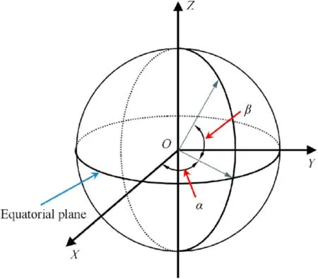
Fig.3.Geocentric equatorial coordinate system.

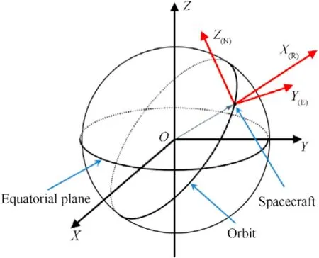
Fig.4.Local coordinate system.

The engineering model of space debris is described by the flux described in Fig.5,and the flux is defined in the local coordinate system;the spatial location is described by orbital elements.Much smaller than its projection on the local horizontal plane,the horizontal component of space debris flux on the x-axis is ignored and only the projection on the local horizontal plane is considered.

In the Y(E)O(S)Z(N)plane,the direction of the flux is discretized into 36 intervals,with[0,360°)equally divided in steps of 10°,and taking the median as the sampling point.The velocity of the flux is generally discretized into 22 intervals,with [0,23] km/s divided equally by 1 km/s step,and taking the median as the sampling point.

The main space debris environment models are:NASA's ORDEM[11] series,ESA's MASTER [12] series,RKA's SPDA [13] series and Harbin Institute of Technology's SDEEM [14] series.The ORDEM model is based on space-based detection data and only includes space debris data,while the MASTER model is based on theoretical models,including space debris models and micrometeoroid models.And the micrometeoroid environment models mainly include the Course-Palais model,the Grün model [15] (NASA SSP-30425) and the Divine model.Among them,the Cours-Palais model is the least used;the Grün model is the most widely used,and the Divine model has been integrated into the MASTER model.

Since RKA's SPDA series are not open to the public and the US only discloses the ORDEM2000 model,this paper mainly uses ORDEM2000,MASTER8 and SDEEM2015 as the input source for spacecraft sensitivity assessment.

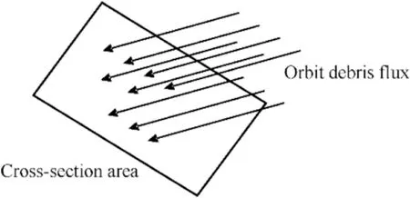
Fig.5.Definition of space debris flux.

3.2.1.ORDEM2000 and SDEEM2015 models

The modeling methods between ORDEM2000 and SDEEM2015 are different.ORDEM2000 is a low-Earth orbit space debris environment model developed by using the catalog data from the US SSN from 1976 to 1988 and the impact data from LDEF.SDEEM 2015 was developed by the Space Debris High-Speed Impact Research Center in HIT.The operation interface is shown in Chinese.The model is based on a semi-deterministic analysis of a reference population derived from the simulation of all major space debris source terms.The data sources used in modeling mainly include:ground-based or space-based detection data,the space debris sources based on ground simulation tests and theoretical analysis,as well as the historical data collected by relevant space missions.

But the main functions and operation of the two software are similar,and the output file format is also roughly the same.In SDEEM 2015,the generated space debris data file divides the size of the debris into 5 groups:>10 μm,>100 μm,>1 mm,>1 cm,and>1 dm;the velocities from 0.5 km/s to 22.5 km/s are divided into 23 sections at interval of 1 km/s;the velocity direction from-175°to 175°is equally divided into 36 sections at 10°intervals.The difference between the two software in defining debris is that ORDEM adds a group of >1 m when dividing the debris size.

3.2.2.MASTER8 model

MASTER8 is a space debris environment engineering model developed by ESA.The function and operation interface are quite different from the above two software.The output file of independent variables can be customized,but it is also more complex to operate,and the debris size needs to be manually set for output.To facilitate the input of sensibility calculations,the “impact azimuth angle-impact velocity”is selected as the space debris data and the“impact elevation angle-impact azimuth angle” is selected as micrometeoroid data.Define the velocity output interval to 1 km/s and the angle output interval to 10°.

The velocity of space debris is output with the range from 0 to 23 km/s,and the velocity of micrometeoroids is output from 0 to 50 km/s.The data of each debris size range is a separate output file.The velocity,size and direction of the space debris data are the same as that in SDEEM2015.The direction of micrometeoroid data is from-90°to 90°and is divided into 18 sections with an interval of 10°,and the azimuth is divided into 36 sections with an interval of 10°from-175°to 175°,with a total of 18 × 36 directions.

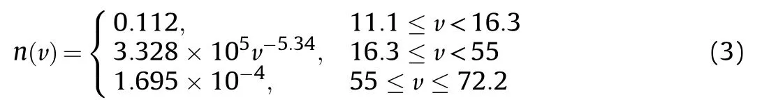
The data output of micrometeoroid from MASTER8 is a flux with a certain direction and size range,and there is no discretization of velocity,so it is necessary to discretize the velocity of micrometeoroid data before using it.Here we use the rate distribution function of NASA SSP-30425B micrometeoroid model in Equation (3),and the distribution is shown in Fig.6.

4.MM/OD data processing based on PCHIP

4.1.Piecewise cubic Hermite interpolating polynomial

First of all,the PCHIP [16] can well overcome the problem of Runge phenomenon;in addition,compared with the cubic spline interpolation method,it can ensure the monotonicity of the fitted curve.

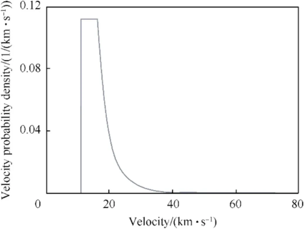
Fig.6.Velocity probability density distribution of micrometeoroids with velocity.

Construct a piecewise cubic Hermite interpolation polynomial.Assume that on the node a=x0≤x1≤x2···≤xn=b,yi=f（xi）,mj=f'（xj）,j=0，1， ···， n,if the function In（x） satisfies the condition:

(1) In（x）∈C1［a，b］;

(2) In（xj）=fj，I'n（xj）=mj，j=0，1，2，…，n;

(3) Each interval ［xk，xk+1］（k=0，1，2，…，n-1） is a cubic polynomial

Then In（x） is called the piecewise cubic Hermite interpolation polynomial.If it is expressed by the interpolation basis function,the expression of In（x） in the entire interval ［a， b］ is:

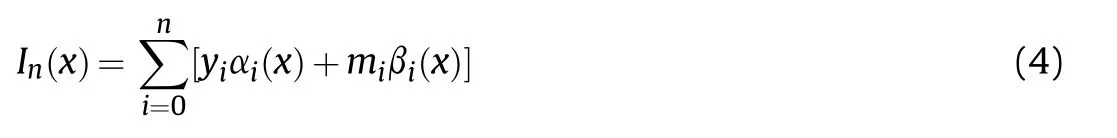
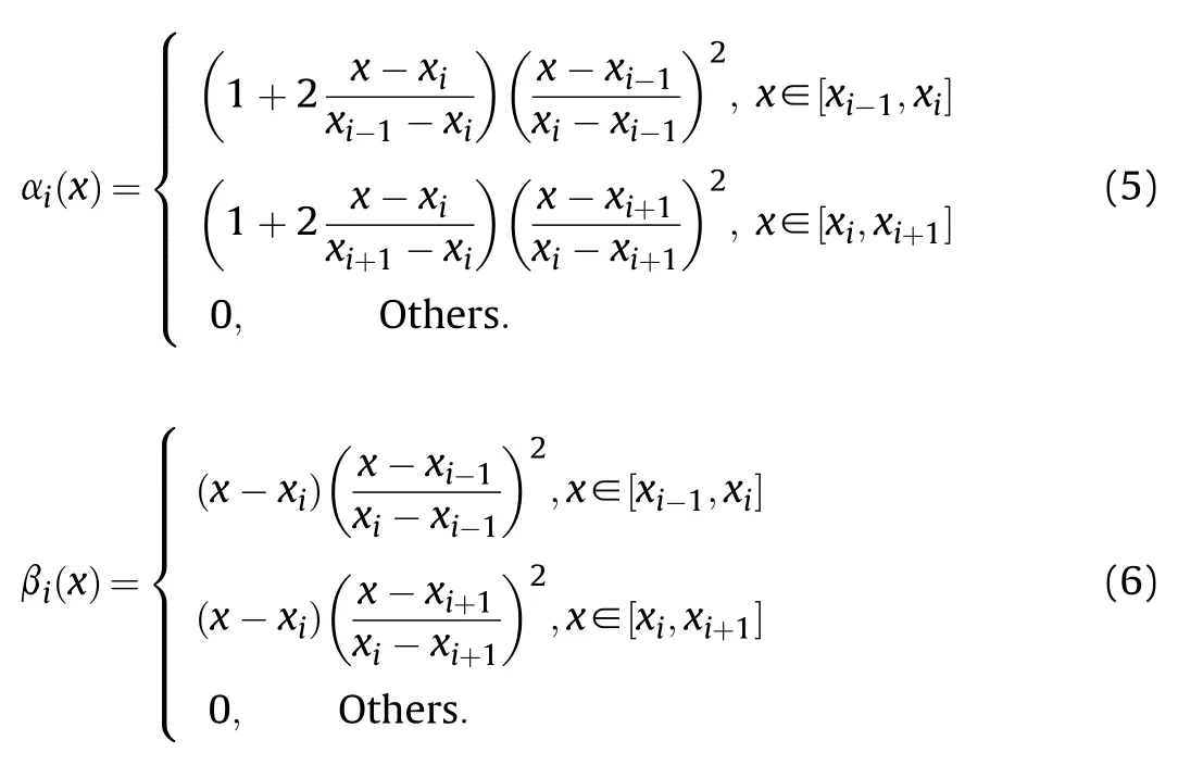
The αi（x） and βi（x） in the interpolation basis function are:

4.2.MM/OD data processing

The file formats are different among the three space debris environmental engineering models used in this paper,which thus need to be unified for subsequent calculations.A finite element sphere is used to characterize the impact flux of the spacecraft encountering MM/OD in various directions.Taking the orbit of the International Space Station as an example,the parameters are shown in Table 1.The three space debris environmental engineering models are used to calculate the MM/OD flux data for subsequent input and processing.The results are shown in Table 2.

The debris data from the environmental engineering model is obtained in groups of >10 μm,>100 μm,>1 mm,>1 cm,and>1 dm,as shown in Table 2.Although the MASTER8 and SDEEM2015 can generate debris data with more sizes,they fail to interpolate and fit the data.However,in order to get the MM/OD flux of any size interval,the discrete data must be interpolated and fitted.ORDEM2000 performs a cubic spline interpolation,while ESABASE2 interpolates linearly[17].This paper uses the above two methods to fit the debris data from MASTER8 and SDEEM2015 and compares the result with their original data.The results are shown in Figs.7 and 8 respectively.

There are large gaps between the data output from the engineering model and the results of cubic spline interpolation shown in Figs.7 and 8,whose results in 10 μm-100 μm are non-monotonic and therefore not correct,because the actual output from the space debris engineering modeling software is in accumulative distribution instead of the non-monotonic distribution.Yet as shown in Fig.9,the original data in ORDEM is already processed through the cubic spline interpolation,so there is no case where the curve is non-monotonic.

As illustrated in Fig.7,while the results from both the Linear interpolation and the PCHIP are similar to the original data of MASTER8,the data from 10 μm to 200 μm represented by PCHIP is comparatively more matched with the original data.As shown in Fig.8,there exist relatively large errors between the results from Linear interpolation with those from the original,especially in 10-100 μm and 1 mm-1 cm.From what has been discussed above,this paper adopts PCHIP to obtain the debris flux of any size.

Figs.10-12 are the pseudo-color diagrams of the impact flux from all directions in ORDEM2000,SDEEM2015 and MASTER8,respectively.

Since the data input by MASTER8 includes the data flux of micrometeoroids and space debris,in the subsequent analysis,the data of micrometeoroids and space debris can be analyzed separately.The pseudo-color maps of the impact flux from meteoroids and space debris in all directions are shown in Figs.13 and 14 respectively.

5.Sensitivity analysis of spacecraft based on the panel method

5.1.Impact sensitivity analysis method of spacecraft

The impact sensitivity of spacecraft components refers to the possibility of spacecraft components impacted by space debris.The impact sensitivity of each component of a spacecraft impacted by space debris or secondary debris is characterized by the probability Ph.

The flux F is known as the number of space debris passing through a unit area per unit of time under specified parameter range.Given the duration t of the task,the expected value λ of the space debris passing through the cross-sectional area with an area of S can be expressed as

Assuming that the event of space debris hitting a spacecraft meets the Poisson distribution [18],the probability of k impact events P (n=k) is:

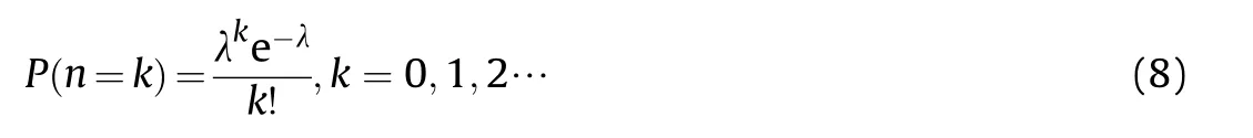
Among them,n is the impact number;λ is the expected number of impacts;P is the corresponding probability.From the formula,the probability P (n=0) that the impact will not occur is:

The probability of at least one impact is:

5.2.Spacecraft motion model

As the distribution of space debris changes with time and space,the spacecraft will encounter different space debris when operating in different orbits.And since the spacecraft operates in different attitudes,the impact of space debris on each part of the spacecraft will also vary.Both the orbit and the attitude of spacecraft affect the safety and reliability of its orbiting operations.This section mainly discusses the kinematic description of spacecraft attitude and orbit and its application in spacecraft impact sensitivity [19].

5.2.1.Definition of coordinate system

The geocentric inertial coordinate system OXiYiZi,the orbit coordinate system OXcYcZc,the body coordinate system OXbYbZb,and the velocity coordinate system OXvYvZvare used in this paper.And the geocentric inertial coordinate system has been described in section 3.1.

1.The orbit coordinate system OXcYcZc

As shown in Fig.15,the origin is at the mass center of the spacecraft;the Xc-axis is along the intersection between the orbital plane and the local horizontal plane,and points to the forward direction of the spacecraft;the Zc-axis points to the center of the earth along the local vertical line,and the Yc-axis is determined by the right-hand rule.

2.The body coordinate system OXbYbZb

The origin is located at the mass center of the spacecraft,and the three axes of the coordinate system are the inertial principal axes of the spacecraft.

3.The velocity coordinate system OXvYvZv

As shown in Fig.16,the origin is at the mass center of the spacecraft;the Xv-axis is the relative velocity vector direction of thespacecraft;is the vector of a spacecraft's mass center pointing to the earth center;Zvpoints to×,Yv-axis is determined by the right-hand rule.

Table 1 Orbital parameters of spacecraft.

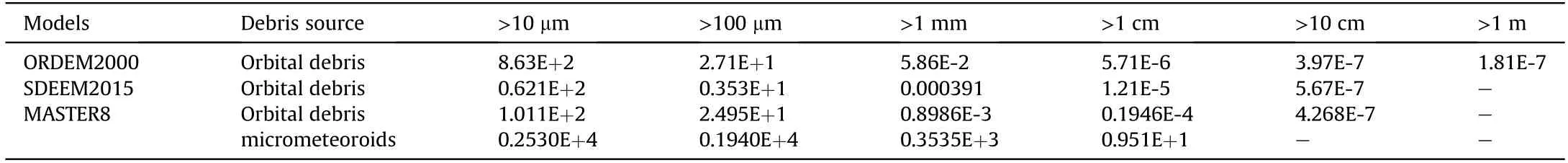
Table 2 MM/OD flux data with different sizes in three models.

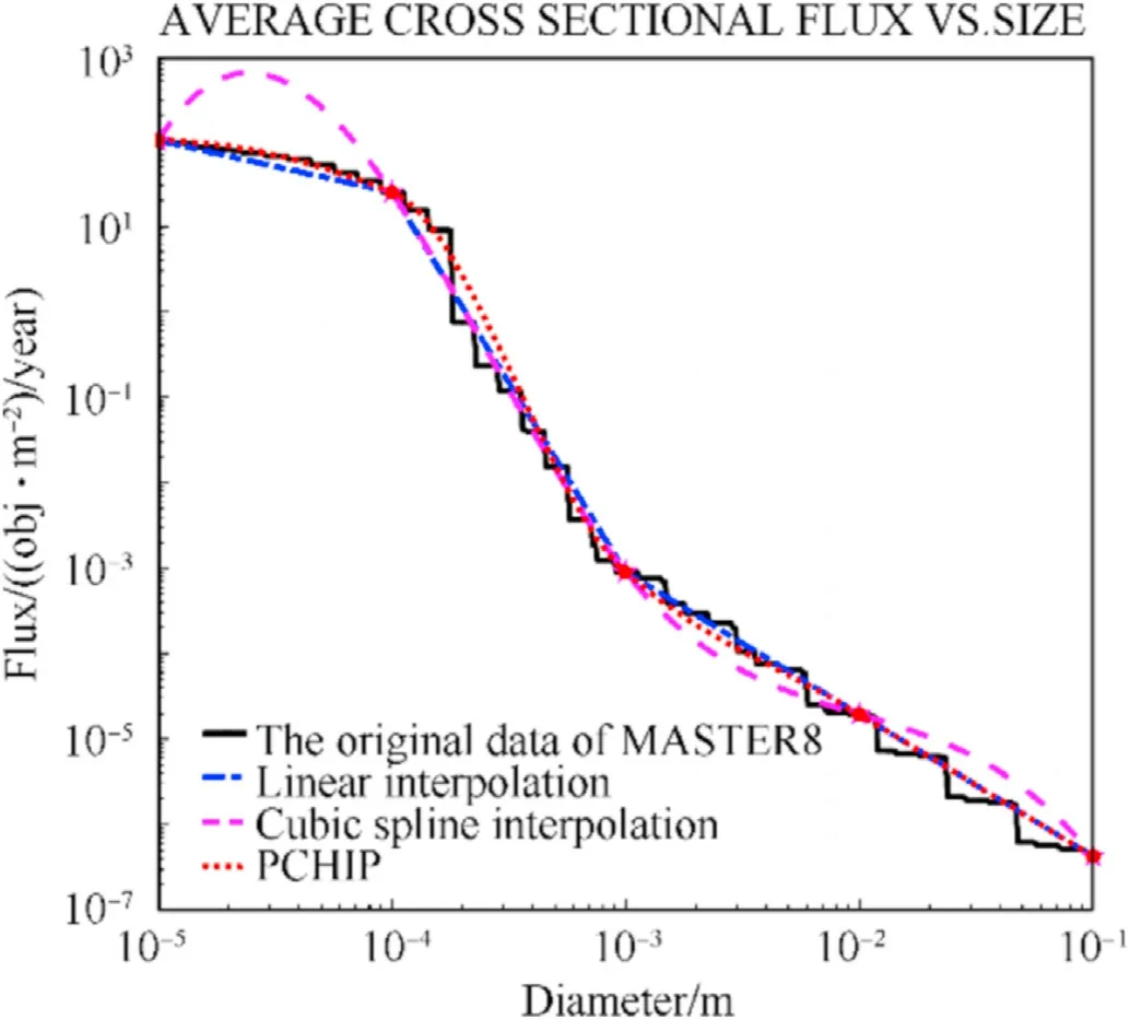
Fig.7.Comparison of three different interpolation methods with MASTER8 original data.

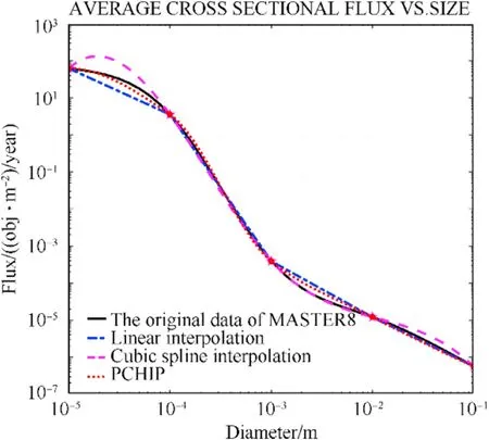
Fig.8.Comparison of three different interpolation methods with SDEEM2015 original data.

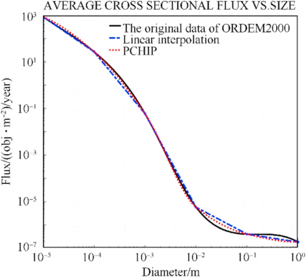
Fig.9.Comparison of two different interpolation methods with ORDEM2000 original data.

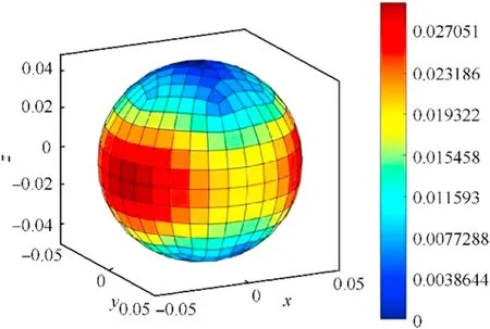
Fig.10.ORDEM2000.

To study the impact effect of space debris on spacecraft,the space debris inflow coordinate system is established,which is defined as:the origin is located in the mass center of the spacecraft;Xlshows the inflow direction of space debris,Zlpoints to×;is the relative impact velocity of space debris to the spacecraft.is the geocentric vector of the spacecraft;Ylis determined according to the right-hand rule.

5.2.2.Spacecraft attitude model

The geometric modeling of spacecraft is generally carried out in the body coordinate system,while the impact threat direction generated by the space debris environment model is defined in the orbital coordinate system[20].Therefore,the spacecraft geometric nodes must be converted to the orbital coordinate system according to the spacecraft attitude transformation.

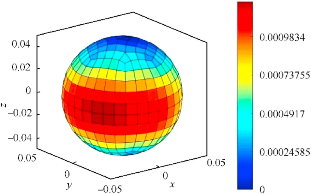
Fig.11.SDEEM2015.

Fig.12.MASTER_MMOD.

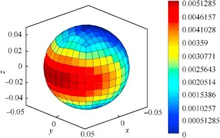
Fig.13.MASTER_Orbital Debris.

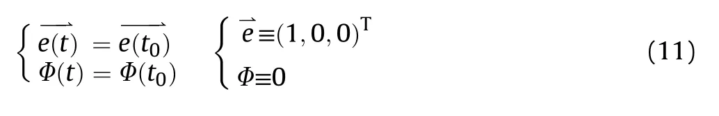
Make the reference coordinate system OXYZ,and the body coordinate system is OXbYbZb.Suppose the Euler axis is=（ex，ey，ez）and the angle of rotation is φ,at time t0:（t0）==（ex0，ey0，ez0）,φ（t0）=φ0.The impact of the two attitudes on spacecraft impact is discussed.

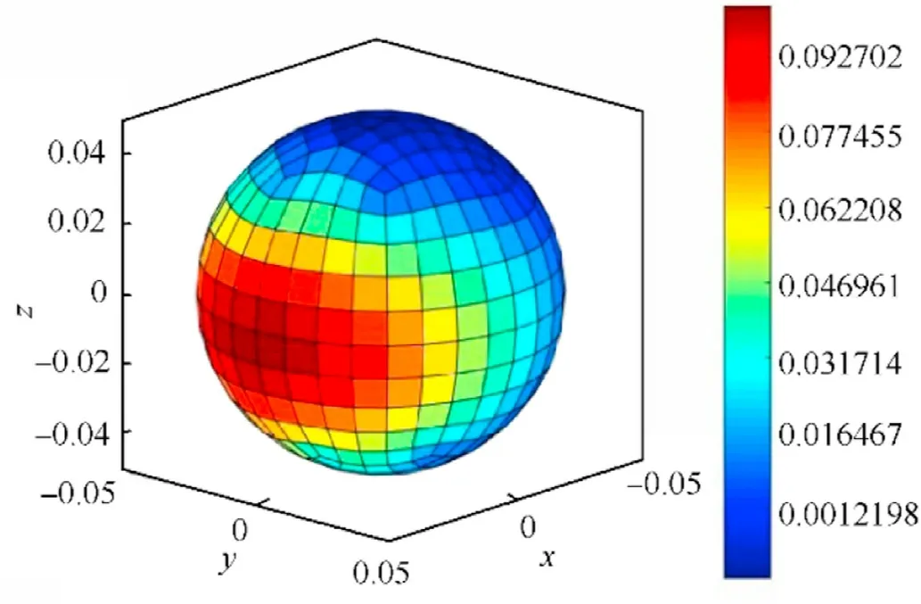
Fig.14.MASTER_Micrometeoroids.

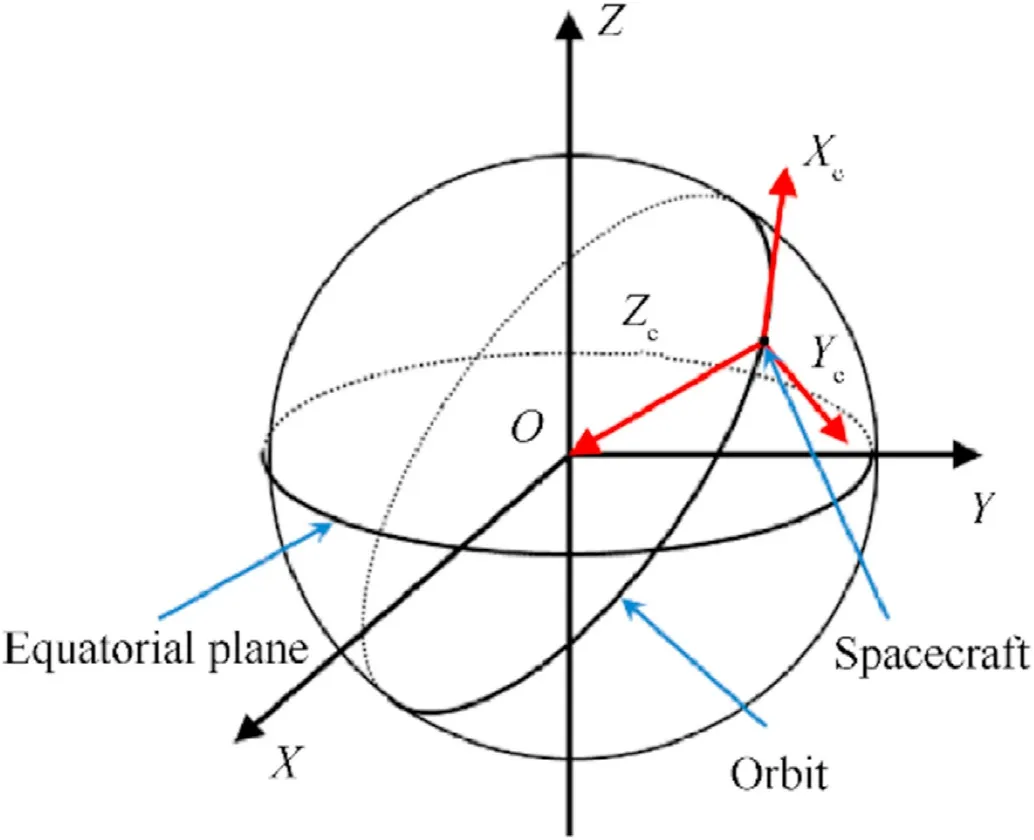
Fig.15.Orbit coordinate system.

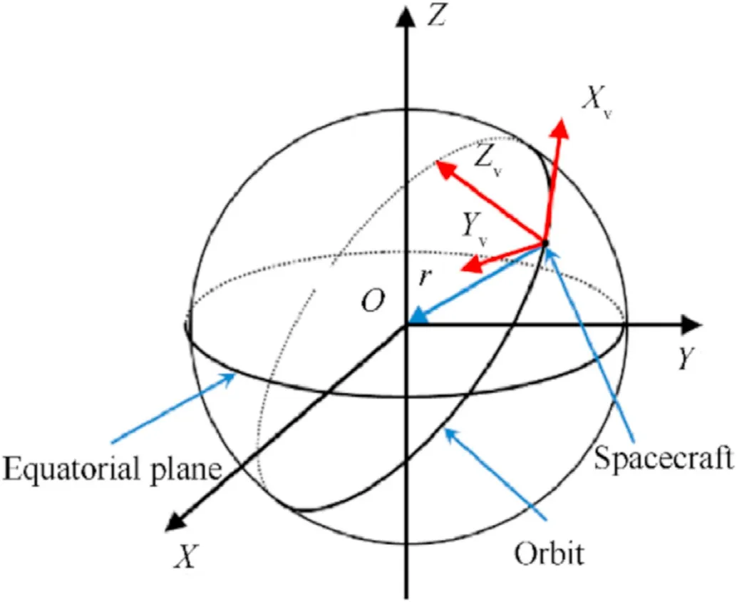
Fig.16.Velocity coordinate system.

1.Three-axis stability: The Euler axis and angle parameters are constants.In this paper,the X-axis unit vector is used,and the angle parameter is 0

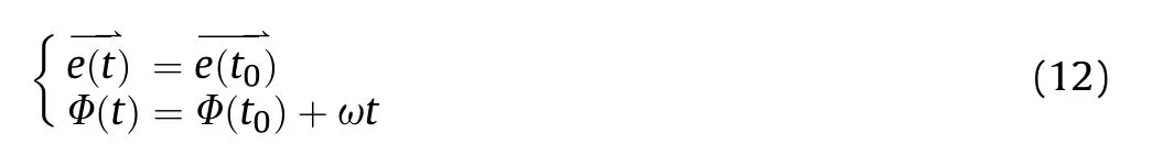
2.Spin stability: Assuming the angular velocity of rotation is ω,then the posture at any time is expressed as:

The attitude of fixed-axis rotation changes with time in the reference coordinate system,and the time relative to the perigee moment is:

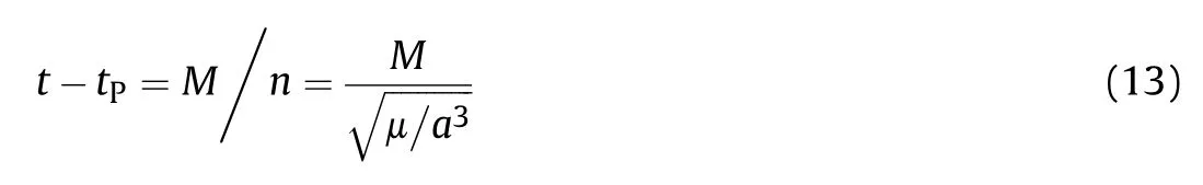
where tPis the moment of passing perigee.The time relative to the initial point is:

Fig.17.Diagram of coordinate transformation.

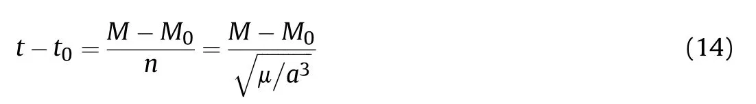
where t0is the initial moment.The initial Euler axis is set toand the rotation rate is ω0,then

As shown in Fig.17,take Euler angle according to the initial state of the spacecraft attitude as: ψ,θ,φ.According to Rodrigues formula,the initial coordinate in orbital coordinate system is A0=（x0，y0，z0）,and the coordinate Abrat time t can be expressed as:

Among them,the transformation matrix R（，φ） is:

5.3.Spacecraft shielding analysis

The spacecraft shielding happens between the spacecraft's protective structure and the inner and outer components,which refers to the shielding of different components of the spacecraft on the path of space debris impact.Similar to light propagation,for a specific inflow direction of space debris,the components in the front will block and prevent the components behind from being impacted.Each component is subjected to different impact probability from space debris as a result of the shielding between components and the unpredictable distribution of space debris,so taking the shielding into the consideration plays a significant role in spacecraft vulnerability assessment.

5.3.1.Shielding algorithm

As shown in Fig.18,in the inflow direction of the space debris,the component A behind the protective structure is blocked by the component B.The projected area of the component A blocked in the incoming direction is called the blocking area of the component A,which is SAsh.And the projected area of component A exposed to the inflow direction of space debris is called the exposed area of component A,which is SAex,then:

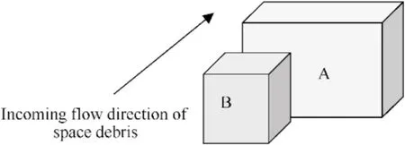
Fig.18.Diagram of component shielding.

ηAis the exposure coefficient of component A.

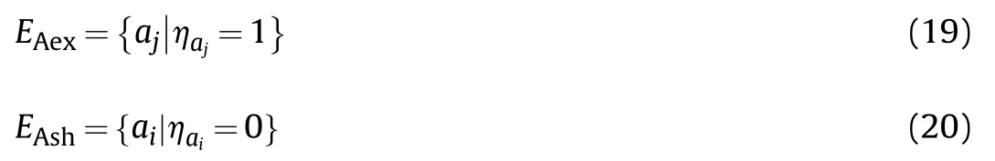
Suppose the elements collection of component A are EA,EA=｛aj∈E|j=1，2···NA｝.Since each element area is small,the shielding states for a certain element ajcan be simplified into two states:fully blocked or fully exposed.When it is blocked by another element,set this element the exposure coefficient ηaj=0;and vice versa,when it is fully exposed,set this element the exposure coefficient ηaj=1.Then the element set of component A can be divided into two groups: the exposed element set EAexand the shielded element set EAsh,which are,

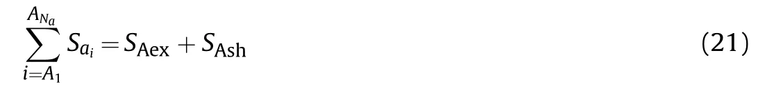
The projected area of component A is equal to the sum of the exposed area plus the shielded area,which is the sum of the projected areas of all elements of component A.

The exposed area of some certain component can be expressed as:

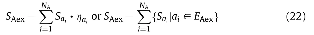
The shielding area can be expressed as:

The exposure coefficient of the component is:

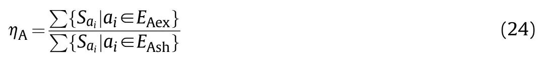
The exposed area and the exposure coefficient of the component are obtained through the analysis of the shielding among each component's finite elements.The exposure coefficient ηaof the finite element is calculated by the shielding algorithm.Using the formula given above,the exposed area,the shielding area and the exposure coefficient of the component are calculated.

5.3.2.Algorithm process

For better analysis of spacecraft vulnerability,this article adopts an improved area-scanning method.The general process of the shielding algorithm is:

Step 1:Identify the rear element,and record the exposure coefficient of all rear elements as 0;

Step 2:After removing all the rear elements from the finite element set of components,the remaining elements are analyzed about their position relationship and depth relationship.Among the elements that are in a position of intersection,enclosure or compatibility,the element with the smallest depth is regarded as the exposed element,and the exposure coefficient is 1,while the element with the largest depth is regarded as the shielded element,and the exposure coefficient is 0;

Step 3:Repeat step 2 and identify all the non-rear elements till all the exposure coefficients are obtained.

1) Identify rear element of the component

The rear element of the component refers to the plane whose angle between its outer normal direction and the inflow direction of space debris is no greater than 90°,and the rest are called the front element.The flow of space debris can be regarded as a line of sight.In this case,the rear element is invisible in the direction of the line of sight,and it will not block the rest of the model,or even when the shielding occurs,the effect will be replaced by the front element.Therefore,the rear element can be removed from the finite element set for analysis,which will not affect the calculation of both the exposed area and the exposure coefficient.

The rear element can be determined by the angle between the outer normal of the element and the direction vector of space debris impact.The judgment method is:setting the outer normal of a certain element as,the direction of the space debris flow;if≥0,the element can be determined as the rear element.

2) Determine the position of the element

The positional relationship among elements is determined on the projection surface of the incoming flow direction,turning the three-dimensional space to the two-dimensional space to simplify the calculation.The positional relationship between finite elements can be divided into four categories,namely intersection,compatibility,separation,and enclosure,as shown in Fig.19.

(1) Determination of intersection

The positional relationship between elements is determined with reference to the element edge lines.If there are at least two projected edge line segments in one element that intersect with those in another element,then the two elements are in a position of intersection.

The calculation method to solve the intersection of the two linesegments will be given below.The two line-segments are represented by L1and L2respectively.The start and end of L1are represented by A（xA，yA）and B（xB，yB）respectively;the start and end of L2are represented by C（xC，yC）and D（xD，yD）,respectively.Then the equations of line segments L1and L2can be expressed as:

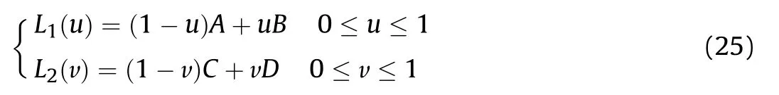
The parameter equation is written as:

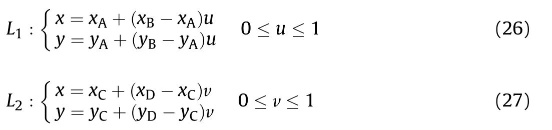
If there is an intersection between two line segments,then

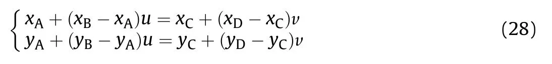
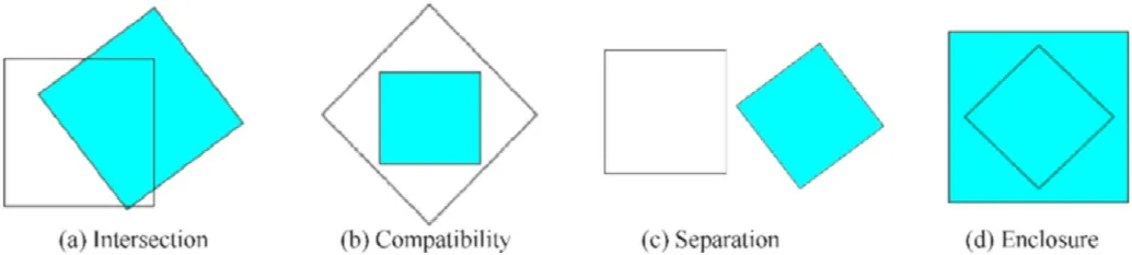
Fig.19.Four positional relationships between finite elements.

The values of u and v through the above formula can be therefore obtained:

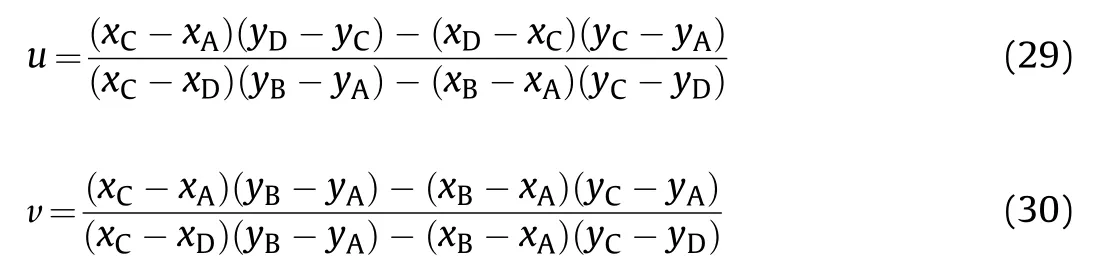
u and v are analyzed under different situations:

a.If the two line segments are parallel,the denominator in the analytical formula of u and v is 0,which is（xC-xD）（yB-yA）-（xB- xA）（yC- yD）=0,and there is no solution for u and v;

b.If there is an intersection point between the two line-segments,then 0 ≤u ≤1 and 0 ≤v ≤1;

c.If the intersection point is on the extension line of L2,then 0 ≤u ≤1 and v<0 or v>1;

d.If the intersection point is on the extension line of L1,then 0 ≤v ≤1 and u<0 or u>1;

In the above four cases,the two line-segments can be determined as intersecting positional relationship only if the conditions 0 ≤u ≤1 and 0 ≤v ≤1 are met.When two or more line-segments in the finite element satisfy this condition,it can be determined that the two elements are in a position of intersection.

(2) Determination of compatibility,enclosure and separation

The three positional relationships including compatibility,enclosure and separation can be determined through the rotation inspection method.Rotation inspection is to make a circle around the element in a certain direction,and the sum of the angles formed by the connection between the two adjacent vertices and the center of the other element is ∑α.If ∑α=360°,the element is in a compatible or enclosing position relationship;if ∑α≠360°,the panel is in a separated position relationship,as shown in Fig.20.

For the above three positional relationships,the elements that have a shielding relationship belongs to compatibility and enclosure,and those having no shielding relationship belongs to separation.

3) Determination of shielding relationship

Since this paper divides the spacecraft geometric model into small panels for analysis,in the direction of the space debris flow,the positional relationship between the units is intersection,compatibility,and enclosure,so it is considered that there is occlusion between the panels.In the space debris flow coordinate system,the space debris impact direction is set to the+x direction,the element with the smallest x coordinate value is the exposed element,and the exposure coefficient is 1,while the element with the largest x coordinate value is the shielded element,and the exposure coefficient is 0.The in-between elements must continue to be analyzed and then to determine its exposure coefficient.

Through the shielding algorithm,not only the exposed area of a spacecraft in a certain inflow direction of space debris can be calculated,but also the element sequence under the successive impact by space debris can be obtained based on the x coordinate value of each shielded element.The analysis of secondary shielding between elements is realized.

5.3.3.Algorithm implementation

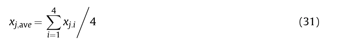
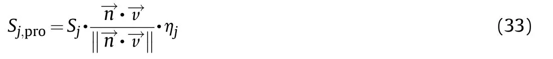
In the space debris flow coordinate system,the vertex of the j-th element is denoted as Vj，i=（xj，i，yj，i，zj，i）,j=1，···，n,i=1，···，4.The outer normal direction of the element is,and the unit vector of the space debris flow direction is.

In this article,the concept of the x-coordinate of the element is proposed.The average of the x-coordinate values of the four nodes constituting the element is obtained as follows:

Given the coordinates of the four nodes of the element,the area of the element is:

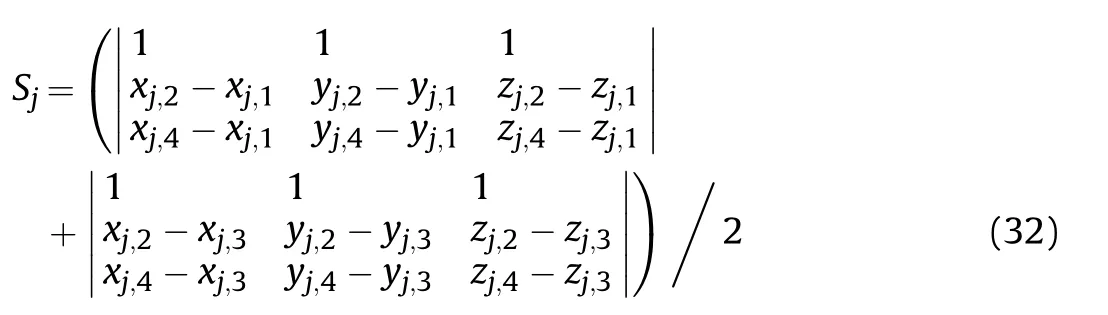
ηjis the exposure coefficient of the j-th element,and the exposed area of the element in the incoming flow direction is:

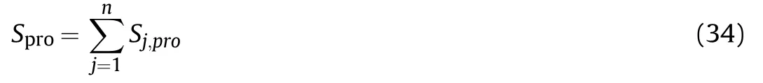
The sum of the exposed areas of all the elements that make up the component is the exposed area of the component.

1) Outer shielding of spacecraft

Outer shielding of spacecraft refers to the shielding between the spacecraft's protective structure and external components.The spacecraft's protective structure and its external components are the top concern when impacted by space debris.It is assumed that the finite element set of the spacecraft protective structure and external components is Esh=｛e1，e2， ···， en｝,and there are n panels in total.The process of the shielding algorithm is realized as follows (see Fig.21):

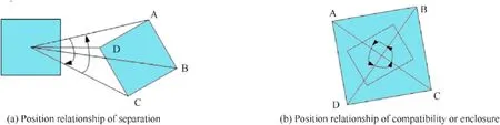
Fig.20.Diagram of rotation inspection method.

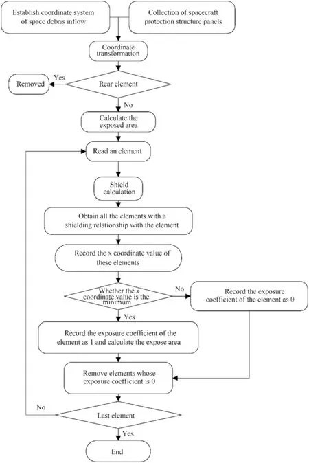
Fig.21.Spacecraft outer shield calculation process.

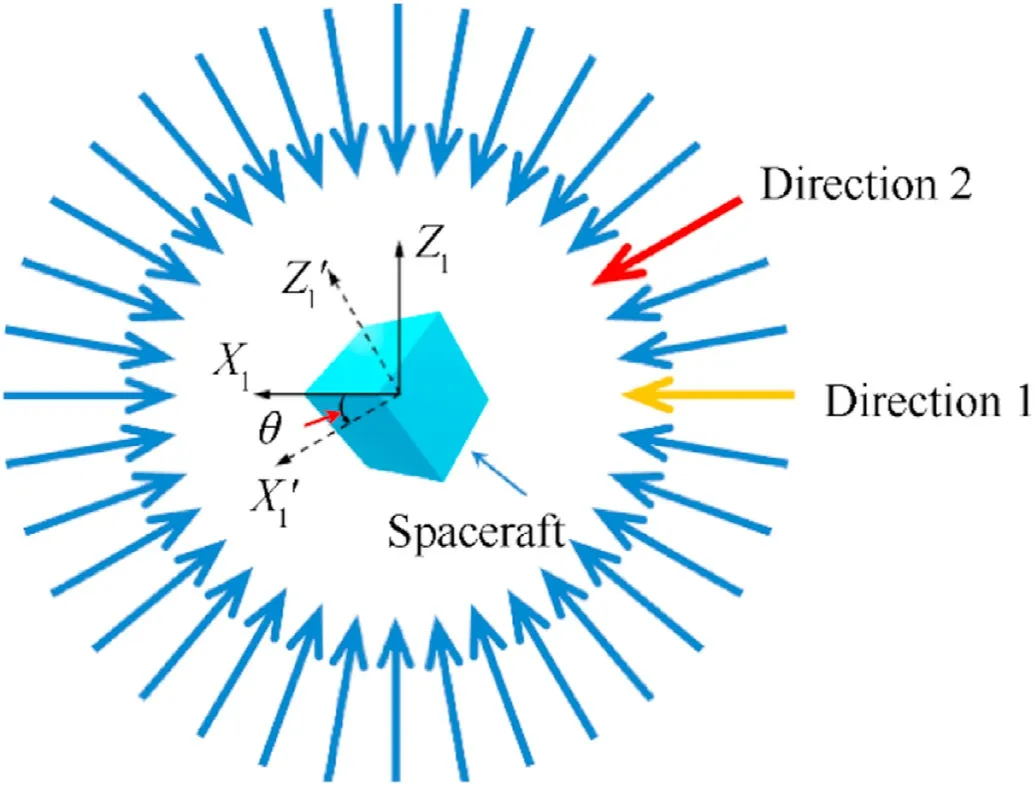
Fig.22.The inflow coordinate system.

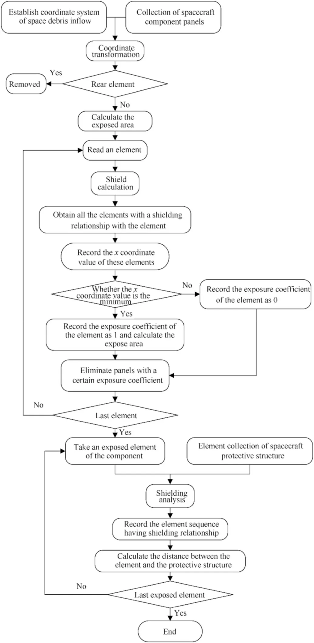
Fig.23.Spacecraft internal shielding analysis process.

The debris from each direction should be individually analyzed.To facilitate the calculation,the inflow coordinate system is established for the debris from all directions.As is depicted in Fig.22,for instance,two coordinate systems XlOZland Xl'OZl' are established to help analyze the debris from direction 1 and 2.Therefore,after determing some certain direction,the spacecraft geometry model is correspondingly converted to the incoming flow coordinate system by Rodrigues formula,through the shielding calculation to obtain those mutual-shielding panels.The panel with larger x-axis data is blocked by that with smaller x-axis data.Take the exposure coefficiency of the smallest x-axis data as 1 and remove those blocked panels.

2) Internal shielding of Spacecraft

The internal shielding of spacecraft refers to the shielding between the internal components of the spacecraft.The shielding relationships both among different parts and between the parts with the protective structure are all need to be analyzed,which are different from that of the outer shielding.The whole process of the shielding analysis is illustrated in Fig.23.The shielding relationship between components is firstly analyzed in a way similar to that for the outer shielding.The inflow coordinate system is then established for debris from each direction.And through shielding analysis,the exposed panel sets of the components can be obtained.Then in the same way,the shielding between the exposed panels of the components and the protective structure is then analyzed.The panels in shielding relationship will be recorded and the distance from the component panel to the protective structure panel will also be recorded and calculated for subsequent vulnerability analysis.

This article mainly studies the primary shielding of the protective structure and ignores the secondary impact of the debris cloud generated on other components.

5.4.Sensitivity calculation

After the shielding calculation,the shielding relationship between the two outermost layers is obtained.But the calculation methods for the impact probability of the two outermost layers are different.The outermost panel element is the protective structure,which directly encounters the impact of MM/OD,yet the particle impacting the second layer panel element must first penetrate the first.So,the number of impacts on the second layer panel element can only be obtained through the calculation of the impact limit on the first layer panel element.Only particles larger than the limit size can pass through the first layer element to reach the second layer.The limit size of the surface element of the protective structure is calculated with the impact limit equation.Three most commonly used limit equations are listed in this paper:

(1) Impact limit equation of single-layer plate

The current most widely used impact limit equation of singlelayer plate is the improved Cour-Palais equation [21]:

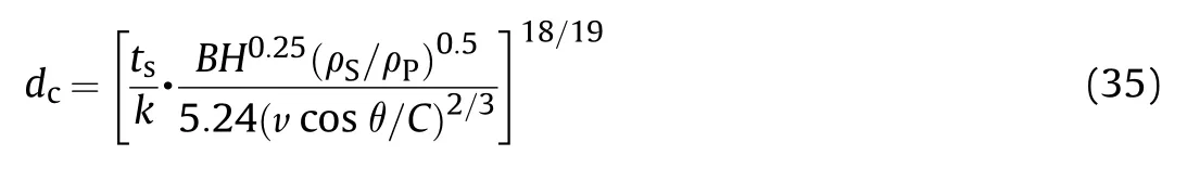
where dcis the critical fragment diameter;BH is Brinell Hardness;tsis the thickness of target plate;ρSand ρPare respectively the density of the target plate and the projectile;C is the sound velocity of target plate;v is the fragment velocity;θ is the impact inclination angle and k is 1.8.

(2) Impact limit equation of Whipple protective structures [22]

Whipple protective structure is a typical protection scheme of orbit debris,which includes two layers of metal plates.The first layer is a buffer structure.After debris impact,secondary debris clouds are generated,and secondary debris clouds expand along the velocity direction and impact on the bulkhead.As the action area increases,the energy is dispersed and the damage to bulkhead is effectively reduced.Christiansen equation is the most widely used impact limit equation for double-deck plates:

where subscript b and w represent the parameters of the first layer and the second layer respectively;t is the thickness of the plate;ρ is the density,and σ is the yield strength of the back wall.

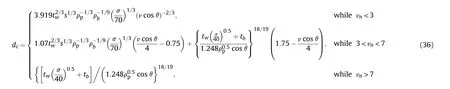
(3) Impact limit equation of Honeycomb sandwich panel [23]

Honeycomb sandwich panel is a widely used protective structure on satellite.It can be seen as a combination of Whipple structure and aluminum honeycomb core.Under high-speed impact,the front panel of honeycomb sandwich panel is broken and moves radially.Honeycomb core absorbs energy through plastic deformation,rupture and disintegration,which hinders the radial movement of debris cloud.

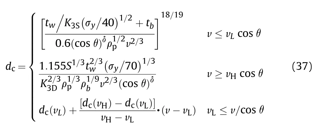
Among them,the corresponding parameters of the honeycomb structure of different materials are different,as shown in Table 3:

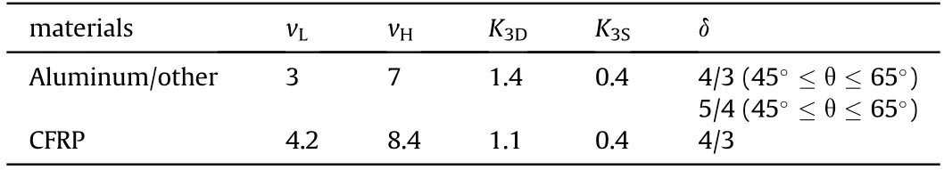
Table 3 Parameters of impact limit equation for honeycomb structures.

5.4.1.Sensitivity calculation example

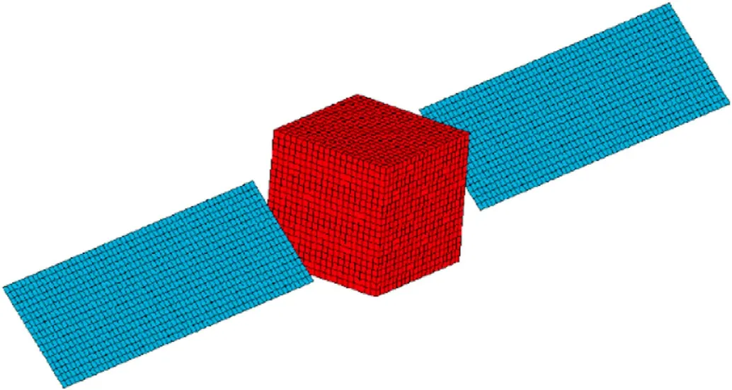
Fig.24.Model 1.

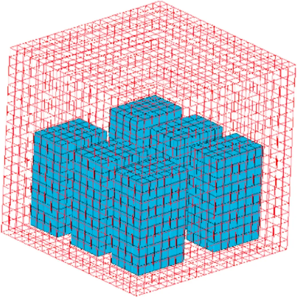
Fig.25.Model 2.

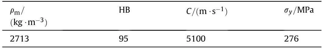
Table 4 Material properties for aluminum Al-6061-T6.

In this paper,two simplified satellite models were used to verify the feasibility of the outer and the inner shielding algorithms respectively.The shielding for one cubic satellite with a side length of 1 m and two 3 × 0.85 m solar arrays was analyzed in Fig.24 Model 1,and each solar array was equivalent to a 0.05 cm aluminum Al-6061-T6.In Fig.25 Model 2,the 1 m long cubic star blocks six 0.2×0.3×0.5 m battery packs inside,and the exterior of the cubic satellites equals a 0.3 cm Aluminum Al-6061-T6.The characteristics of the material are listed in Table 4 [24].

The mission considered is a one-year mission in a SSO with altitude equal to 802 km,inclination of 98.6°,and eccentricity of 0.001 with starting epoch on the 1st of January 2016.Take the data respectively calculated by SDEEM2015 and MASTER-2009 as input for calculation,and then compared the results with ESABASE and DRAMA.

From the calculation results in Fig.26,there is obviously mutual shielding between the solar array and the cube satellites,which verifies the spacecraft's external shielding algorithm.Comparing Fig.26-a with Fig.26-b,judging from the number of impacts on the outer surface of the cube satellites,the number of debris by SDEEM2015 are more evenly distributed,scattering on the front,left and right sides of the cube,while the debris output by the MASTER-2009 model concentrated in the front of the cube,the number on the left and right sides is small,and there is few at the back.

From Table 5,it can be seen that the calculation results in this paper are consistent with the results of ESABASE2 [24],but are different from those calculated by the DRAMA model [24].This is because ESABASE2 also uses the MASTER-2009 population as the debris source input,and the idea of SDEEM2015 model is similar to that of MASTER-2009 model.Yet the debris source used in DRAMA is ESA-MASTER.In terms of the impact numbers on the battery,the SDEEM2015 has a slightly smaller number,indicating that for this test case the percentage of large-sized debris in the SDEEM2015 population is small.Comparing Fig.28 with Fig.30,in cases of SDEEM2015 as the debris source,the impacts on the battery mainly scatters evenly on the front,left and right,while taking MASTER2009 as the debris source,the impacts on the battery is concentrated on the front.This further explains the differences between the two space debris engineering models(see Figs.27 and 29).

6.Simulation verification of standard working conditions

To encourage the development of risk assessment research,IADC worked on the comparison and verification of space debris risk assessment codes[25].IADC stipulated three standard working condition models,including the same geometric shape,protective structure,and operating parameters.Several different codes were used to evaluate and calculate the risks under the same space debris environment model.The results obtained are compared and analyzed.

Three standard working conditions are specified in the protection manual of space debris,namely,cube satellites,spherical satellites and simplified space stations.The size of the cube satellite is 1 m×1 m×1 m.The cross-sectional area of the spherical satellite is 1 m2.The simplified space station consists of one cube(the size is 1 m × 1 m × 1 m) and three cylinders (the diameter of the three cylinders is 1 m,the length of the cylinder on the-X axis is 3 m,the length of the cylinder on the+Y axis is 2 m,and the length of the cylinder on the-Y axis and on the+Z axis is both 1 m).As shown in Fig.31,it is the diagrams of the three standard working conditions.

Under standard operating conditions,the method adopted in this paper is compared with the results of other risk assessment software both at home and abroad to verify the correctness of this method.Table 1 is used as the orbital parameters of the spacecraft under standard operating conditions,and the ORDEM2000 space debris environment model was selected to generate the space debris flux,and the on-orbit operation status in the year of launch was analyzed.

Table 6 shows the results of impact sensitivity under three standard working conditions.The total impact number for debris larger than 0.1 mm and larger than 1 cm is recorded.The simulation results are compared with those from BUMPER,MDPANTO and MODAOST.From the results,it can be seen that compared with BUMPER,the maximum error of the impact number in the three standard operating conditions is 3.48%,and the minimum error is 0.78%;compared with MDPANTO,the maximum error of the impact number in the three standard operating conditions is 3.24%,and the minimum error is 0.98%;compared with MODAOST,the maximum error of the number of impacts in the three standard conditions is 3.3%,and the minimum error is 0.98%.Therefore,compared with the three software,the errors of the impact number are all within 5%,which further proves the correctness of the shielding algorithm in the sensitivity analysis method.

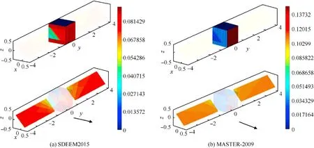
Fig.26.Pseudo-color diagrams of external shielding calculation results under two kinds of debris data input.

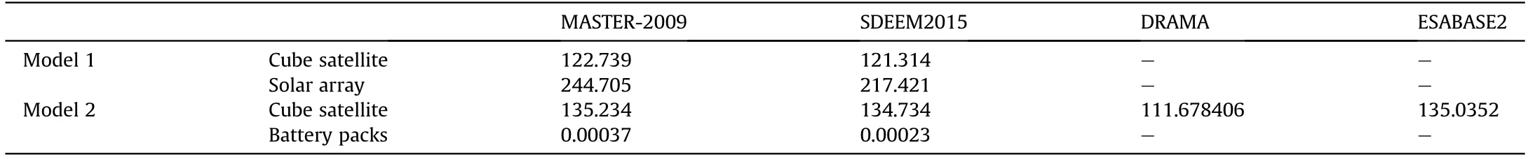
Table 5 Comparison of the impact numbers for a cubic structure.

Fig.27.Pseudo-color diagram of impact effect on cube satellite surface of SDEEM2015 population.

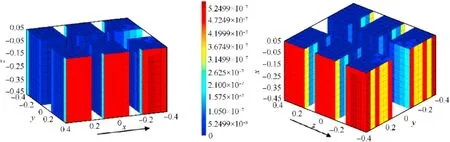
Fig.28.Pseudo-color diagram of impact effect of internal structure of SDEEM2015 population.

From Figs.32-37 are the distributions of the impact number under three standard operating conditions.The direction of the arrows in these figures are the velocity direction of the spacecraft.It can be seen from the pseudo-color diagrams that the number of impacts and the number of failures in the three standard conditions are symmetrically distributed along the forward direction of the spacecraft;when the space debris and the spacecraft move in the same direction,the number of impacts and failures significantly increase;the number of impacts in the+Z and-Z directions of the spacecraft is 0;when d ≥0.1 mm,the number of debris impacts in the+Y and-Y directions is more than that in the velocity direction;and when d ≥1 cm,the number of debris impacts in the velocity direction is more than that on the+Yand-Y directions;These are all determined by the distribution of space debris flux.

Fig.29.Pseudo-color diagram of impact effect on cube satellite surface of MASTER2009 population.

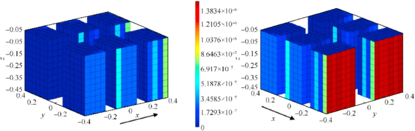
Fig.30.Pseudo-color diagram of impact effect of internal structure of MASTER2009 population.

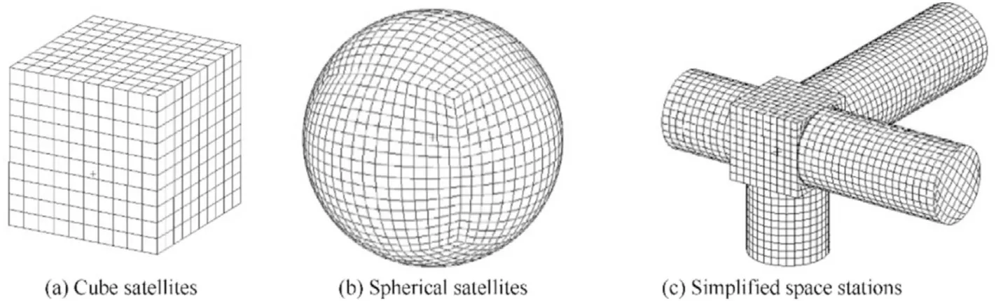
Fig.31.Diagrams of three standard working conditions.

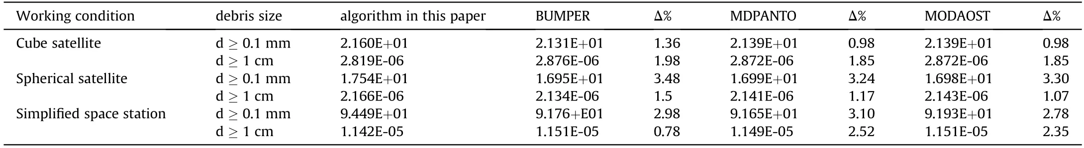
Table 6 Total impact number and impact sensitivity under three standard working conditions.

Figs.32 and 33 are the distribution diagrams of the impact number of the cube.It can be found that the number of impacts on each face of the cube is equal.This is because the exposed areas of the panels on the same face are equal and the normal directions are the same.

Figs.36 and 37 are simplified failure impact distribution diagrams of the space station.It can be seen that for the part on-X-axis cabin that is blocked by the -Y--axis cabin,the number of impacts and failures is less than the rest of the cabin.This also shows that the shielding can effectively reduce the number of impacts.

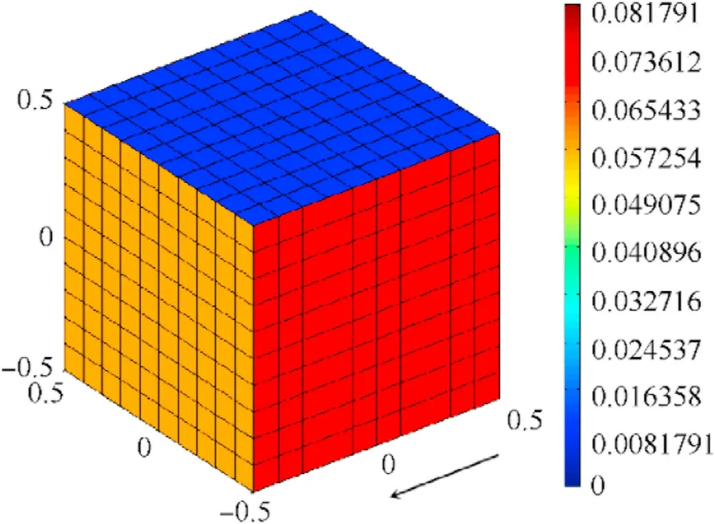
Fig.32.Distribution of impact number on cubic satellite surface (d ≥0.1 mm).

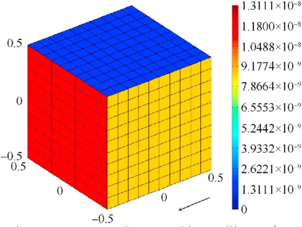
Fig.33.Impact number on cubic satellite surface (d ≥1 cm).

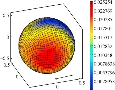
Fig.34.Distribution of impact number on spherical satellite surface (d ≥0.1 mm).

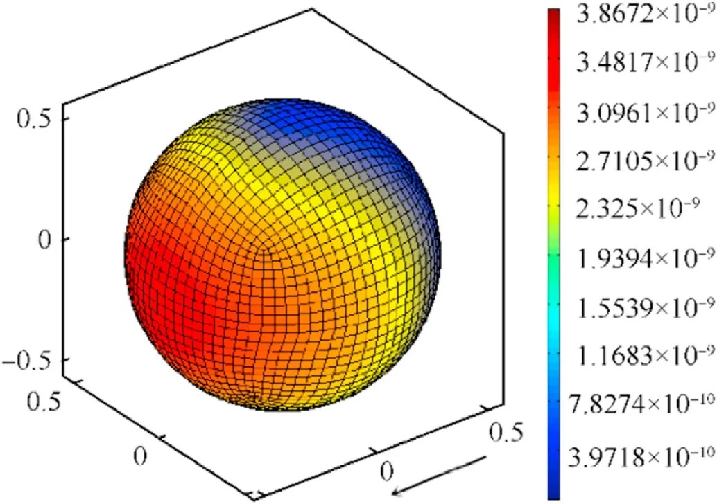
Fig.35.Impact number on spherical satellite surface (d ≥1 cm).

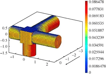
Fig.36.Distribution of impact number on simplified space station surface(d ≥0.1 mm).

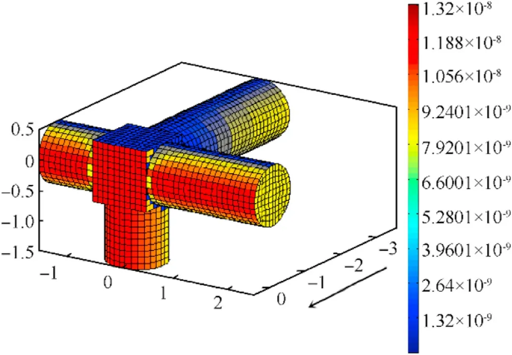
Fig.37.Impact number on simplified space station surface (d ≥1 cm).

7.Conclusions

(1) This paper proposes a calculation method to help predict the sensitivity of spacecraft in the MM/OD environment.An improved panel method is adopted to analyze the mutual shielding between spacecraft components.The spacecraft geometric model is firstly divided into small panels.Based on the shielding analysis between panels,it is determined whether the components are impacted by space debris under MM/OD,the number of impacts on each panel is calculated,and the impact probability of each component encountering debris under MM/OD is obtained through calculation.The feasibility of this method is verified by two simplified spacecraft models,and the “Model 2” test case compared with ESABASE2,the evaluation results are very reliable.

(2) The method presented in this paper integrates three models:NASA's ORDEM2000,ESA's MASTER8,and the SDEEM2015(space debris environmental engineering model developed by Harbin Institute of Technology),and adopts the PCHIP method to interpolate and fit the size-flux relationship of space debris,and compared with ORDEM's cubic spline interpolation and ESABASE2's linear interpolation method,the problems which exist in MASTER8 and SDEEM2015 that the cubic spline interpolation generates inaccurate results are solved.Compared with the results from MASTER8 and SDEEM2015,the method presented in this paper has smaller error.

(3) The standard working conditions of IADC and the sensitivity analysis results of BUMPER,MDPANTO and MODAOST are cross-checked,and the evaluation results are very close to those from the three software,which verifies the feasibility and correctness of the method.

Declaration of competing interest

The authors declare that they have no known competing financial interests or personal relationships that could have appeared to influence the work reported in this paper.

Acknowledgments

This work was supported by the National Natural Science Foundation of China (Grant No.11772113).