Data-driven prediction of plate velocities and plate deformation of explosive reactive armor

Mrvin Becker ,Andres Klvzr ,*,Thoms Wolf ,Meliss Renck

a Institute of Saint-Louis,5 Rue du G′en′eral Cassagnou,68330,Saint Louis,Cedex,France

b Ecole Centrale de Lille,Cit′e Scientifique,59651,Villeneuve d'Ascq,Cedex,France

Keywords:Artificial neural network

ABSTRACT Explosive reactive armor(ERA)is currently being actively developed as a protective system for mobile devices against ballistic threats such as kinetic energy penetrators and shaped-charge jets.Considering mobility,the aim is to design a protection system with a minimal amount of required mass.The efficiency of an ERA is sensitive to the impact position and the timing of the detonation.Therefore,different designs have to be tested for several impact scenarios to identify the best design.Since analytical models are not predicting the behavior of the ERA accurately enough and experiments,as well as numerical simulations,are too time-consuming,a data-driven model to estimate the displacements and deformation of plates of an ERA system is proposed here.The ground truth for the artificial neural network(ANN)is numerical simulation results that are validated with experiments.The ANN approximates the plate positions for different materials,plate sizes,and detonation point positions with sufficient accuracy in real-time.In a future investigation,the results from the model can be used to estimate the interaction of the ERA with a given threat.Then,a measure for the effectiveness of an ERA can be calculated.Finally,an optimal ERA can be designed and analyzed for any possible impact scenario in negligible time.

1.Introduction

With a shift of modern warfare towards classical threats-such as kinetic energy penetrators and shaped-charge jets-the demand for defense systems of mobile platforms increases[1,2].Commonly proposed add-on armor for these threats are bulging armor[3],electromagnetic armor[4],and explosive reactive armor(ERA)[5].This work focus on the latter,which is a sandwich of an explosive between two armor plates.In mobile platforms,the ERA aims to distract or fracture the threat to decrease its penetration capabilities in the main armor.This is supposed to reduce the requirements for the main armor and the overall weight,which improves mobility.The effectiveness of an ERA is highly dependent on the interaction time of the armor plates and the threat.Therefore,the kinematics between ERA and threat have to be optimized.The plate velocity and plate bending depend on the plate sizes,materials,and position of the detonation;the velocity relative to the threat depends on the impact angle and velocity of the threat.In the pre-design of such an armor system,numerical simulations of the whole setup,as well as laboratory experiments,are too timeconsuming to test a large variety of configurations.

In the past,several analytical models have been developed to predict the plate velocity for infinite plates(Gurney[6],Held[7]),and for plates of finite dimensions(Chanteret[8]).These models work well to predict the velocity of the plate.However,they do not take into account the acceleration phase and the ductile behavior of the plate.Data-driven models are currently not only under active research in many civil research domains(financial,medicine,marketing,robotics),but also in defense applications.Besides computer vision and cybersecurity applications.ANNs are also applied to ballistics and blast.Bobbili et al.uses an ANN to determine the ballistic performance of thin plates[9],Shannon[10]predicts hyper velocity impacts and Saxana et al.[11]and Mohr et al.[12]use ANNs to replace constitutive models.In terms of blast loading,Dennis et al.[13]uses an ANN to model blast in an internal environment and Neto et al.[14]uses an ANN for localized blast on mild steel plates.This paper demonstrates that ANNs can also be used to describe the phenomena of plate bending due to explosive loading for various materials.

2.State of the art methodologies

The following section presents the state-of-the-art methodologies to investigate the kinematics in armor development:an experimental approach,analytical modeling,and numerical modeling.

2.1.Experimental investigation

Fig.1 shows the experimental setup.The ERA sandwich(armor material-explosive-armor material)is clamped together and the explosive is initiated with a detonator at the specified position.For the armor material of the ERA,classical passive armor metals are used:AA 7020-T651,Mars®240,Ti6Al4V.Two different sheet explosives are used:PETN-based Formex and PETN+RDX-based Semtex(PI SE M).An overview of the four configurations that were tested to validate the numerical model are given in Table 1.The experiment is observed with flash X-ray images done with a 350 keV X-ray system.The distance from the flash x-ray tubes to the ERA was 2 m,the distance from ERA to the digital image plates was 0.2 m.The time 0 of the experiments as well as of the numerical simulations was the time when the initiation signal for the detonator was given,resp.the initiation point in the numerical simulation was triggered.To be able to correctly correlate the experimental results with the numerical simulations,RP-83 EBW detonators of Teledyne Defense Electronics with a function time simultaneity of 0.125μs are used[15].In the experiments,the time from the initiation signal to the arrival of the detonation front at the tip of the detonator was 8 μs,experimentally evaluated before with a high speed camera with 5e6 f/s.This delay was taken into account for the correlation with the numerical simulation.The trigger times of the X-ray are chosen such that the whole image size is exploited based on the velocity estimation of the plates by the analytical model by Chanteret,explained in the next section.Based on the position of each plate in two subsequent exposures in the X-ray image,the actual plate velocity is calculated.In practice,two representative material points on the plate are selected,evaluated,and the resulting velocities are averaged.

This averaged value is used in the later comparison as the experimental velocity.The velocity computed with this imagebased approach contains uncertainty due to the approximate identification of the same material point in subsequent exposures,the asymmetric acceleration of the plate,and the lack of perspective control.

2.2.Analytical model by chanteret

The plate velocity of infinite plates can be approximated with an analytical formula of Gurney[6].Since in real applications finite plates are used,Chanteret[8]derived a modification that accounts for a finite plate size,or,to be more precise,lateral and edge effects are included.The following paragraph describes first the Gurney equation and then the modification by Chanteret.

Let A be the plate of interest,B be the second plate,and E be the explosive(compare Fig.2).Then,the velocity vAcan be computed by

where Egis the Gurney energy and C1is a constant

The Gurney energy is determined for many common explosives(e.g.,Kennedy[16]).The plates lateral dimensions can be taken into account by the modification of Chanteret,which adds a term C3in the denominator of Eq.(1).

which is defined by

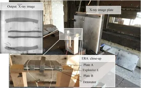
Fig.1.Illustration of the experimental setup:the ERA sandwich is placed on a deformable support in front of an X-ray image plate;a detonator is used to initiate the ERA;a double and triple-exposed X-ray image freezes the dynamics at two/three representative times.

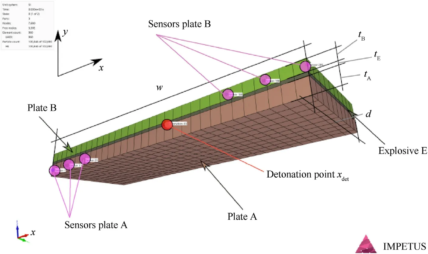
Fig.2.Half-model of an ERA:the explosive is detonated at the detonation point xdet and is cladded between plate A and plate B of size w×d×tii∊(A，B)the displacements are saved for the sensor positions in both plates;the geometries are discretized with finite elements.

where w，d，and tEare width,depth and thickness of the explosive,respectively.

Still,even if the amount of information obtained from the analytical calculation is limited,it is very useful to quickly estimate the plate velocities e.g.for an experimental set-up.On the other hand,the physical basis of the analytical formulation can be used to reduce the input used to train the ANN(model order reduction),as explained in section 3.1.

2.3.Numerical model

The numerical simulations are conducted with IMPETUS;the deformation of the plates is modeled with FEM and the explosive is described with a particle-based approach.Fig.2 illustrates the setup of the simulation.A structured hexahedral mesh with 0.5 mm edge length is chosen for all simulations independent of the plate size(based on a mesh sensitivity study this is sufficient to give good results);the explosive is modeled with 100,000 particles.Thirdorder elements are selected to maintain good approximation properties during large mesh deformation.The elastoplastic plate deformation is accounted for with calibrated material objects:(i)AA7020-T651 by Roth et al.[17],Mars®240 by Nordmetall[18],and Titanium by Meyer[19].The Aluminum and Titanium is modeled with the Johnson-Cook strength model and the Mars®240 with a specific material model for high-strength steels that is only provided in Impetus.None of the material models considers spallation and only a linear equation of state is used,but this has only a marginal effect on the effectiveness of the ERA.

In section 4,the accuracy of the numerical model is validated with the four selected configurations tested for this study.The main purpose of the numerical simulations,however,is to use the sensor data to train the artificial neural network explained in the following section.

3.New methodology:artificial neural network(ANN)for regression

The ANN for this application is developed in the Keras interface of the TensorFlow library[20,21].Keras allows to create a multilayer ANN and to choose the activation and loss function for the model.Here,the ANN is used to perform a regression.The regression approximates the position of a material point of the plate(x0)at a certain time(t)for a given plate configuration.The supervised network is trained with data determined with the numerical simulation.In the following,the training data generation,the data processing,the network architecture,and the training strategy are outlined.

3.1.Generation of training data

A key ingredient of good results with ANNs is a large amount of meaningful training data.In total,the training uses sensor data of 5000 numerical simulations(described in section 2.3).Each simulation models one exemplary configuration in the sevendimensional parameter space(compare Fig.2):material of plate A,material of plate B,thickness of plate A(tA),thickness of plate B(tB),thickness of the explosive(tE),width of the ERA(w),and position of the detonation point(xdet).

Three different armor materials(compare Table 1)take into account design parameters(i)and(ii).In particular,the material density and yield strength of these materials differ,which is important for the variety of the data.The plate thicknesses of each plate(iii)and(iv)are varied between 4 mm and 12 mm;the thickness of the explosive(v)is varied between 1 mm and 5 mm;the width of the ERA(vi)is chosen between 120 mm and 280 mm;the detonation point is located between the center of the plate and 10%from the edge.Within those parameter ranges each simulation is a random pick of all parameters.The plate motion is simulated for 500 μs,which requires between one and 10 min of computation time on the utilized GPU.1NVIDIA Quadro RTX 5000.The license can run ten simulations in parallel,which results in about two and a half days of total computation time for 5000 simulations.More critical is the accumulated data which is-when reduced to the minimum-about 200 GB.Therefore,the required output is saved for 100 material points on both plates with so-called sensors in 5 μs increments.After sorting out the irrelevant part of the sensor data,the size reduces to 7 GB.In summary,all 5000 simulations are evaluated for 100 sensors on each of the two plates at 100 times.This evaluation results in 100,000,000 samples for the training of the ANN.The amount of data points in spatial and temporal direction is further reduced during the optimization of the ANN since some data might be too similar and has marginal influence on the result.This is investigated in section 5.1.

3.2.Processing of the training data

The network approximates the position y of a material point as a function of the seven design parameters described in the last section,its axial position x,and the time t.This results in nine input dimensions,which are not particularly meaningful for the network.By multiplication and other mathematical operations,parameters can be combined and non-linearity can be introduced in the model.E.g.,the ratio between plate thicknesses gives an estimate for the velocity.Furthermore,instead of the material ID,the material density and yield strength of the material characterize the behavior.Finally,this approach reduces the number of input parameters from nine to four(model order reduction).The way to apply the model order reduction has to be chosen carefully,it is in our case based on the physical analysis given by the analytical model.By this,the information which is used to train the ANN is on the one hand reduced,on the other hand only the information important for the result is used.The new input parameters are

·time after the detonation front reached the position(to account for the position of the detonation point),

·position of the plate according to the equation of Chanteret(to add physical information to the model),

·distance to the edge(to account for edge effects),

·relative position on the plate(to account for the size of the plate)

where timeendis the end time of the numerical simulation,and ymaxis the maximum deflection of a material point on the plate.There are dozens of possibilities to choose and normalize the input parameters,but these perform satisfactorily well.At the same time,using the original parameters does not give meaningful results.However,there might be smarter ways to process the input data.This is not further investigated in this work,but might be addressed in future publications.

3.3.Network architecture

Fig.3 illustrates the network architecture exemplary for three hidden layers and 16 neurons per layer.Besides the number of layers and neurons per layer,the architecture is characterized by the activation function of the neurons,the optimizer,and the loss function.The optimizer is used for back-propagating the error concerning the loss function and determines the corresponding weights of each neuron.These weights influence the prediction capabilities for test data unknown to the network.This section describes the choice of architecture and modifications that are compared during the optimization of the ANN.

The right amount of layers and neurons in an ANN is a controversially discussed topic in artificial intelligence.In general,more layers and neurons can improve the accuracy of the method but increase the computational effort.Furthermore,too many neurons and layers can lead to overfitting.Overfitting in terms of artificial intelligence means that the network is very accurate for the training data but inaccurate for test data.The amount of layers and neurons is systematically increased in the optimization procedure until convergence(see section 5.1).

There is limited choice for the activation functions for the application of regression.Based on a literature review the rectified linear activation function(ReLU)is chosen,which has good properties for regression[22].Different solvers implemented in the Keras library can be used,which are,without loss of generality,modifications of a stochastic gradient descent.The ANN uses the Adam optimizer with a root-mean-squared loss to determine the weights via back propagation of the error.

3.4.Training strategy

The training can use the whole data set or only a part of it.In terms of the optimization of the ANN,it is interesting to see how many simulations are needed to give good results.Furthermore,the cropping of the data reduces the time needed for training.During training,the ANN receives a fixed number of training examples as so-called batches.The ANN uses the default of 64 samples in each batch.These batches are not only shown once but several times to the ANN.Each iteration where all batches are presented once is called“epoch”.The error of the ANN is measured by the loss function.When the loss stops decreasing,the ANN weights are converged and the training can be ended.In the optimization of the ANN,the required amount of epochs is investigated.Moreover,the number of simulations and samples per simulation is determined to reduce the training time further.

Fig.3.ANN network structure to approximate the plate position;input dimension is four;three hidden layers with 16 neurons each and ReLU activation;one output layer with linear activation.

4.Step I:analytical,experimental,and numerical results-validation of the database for the ANN

This first part of the results compares the predictions of the state of the art methods.The ANN cannot be better than the data it is trained with-the output of the numerical simulation.So,the question that needs to be answered here,in particular,is how well the numerical model can describe the behavior seen in the experimental results.The four experiments described in Table 1 are used for this evaluation.Since the plate deformation is essential,not only quantitative values but also a qualitative comparison is presented.

4.1.Quantitative comparison between analytical,experimental,and numerical results

Table 2 presents the velocities for the four experiments extracted from the X-ray images(vexp)calculated with the analytical model of Chanteret(vana),and extracted from the Impetus simulation(vnum).Since the experiments reveal the velocities for both plates,there are eight cases to compare.As can be seen in the table,the analytical and the numerical model predict similar values for the plate velocity for most cases.Only in experiment number three,both plates are about 10% faster in the numerical simulation than computed with the analytical model.On average,the predicted plate velocity of the analytical and numerical model is 5% smaller than the value extracted from the experiment.The worst prediction of the analytical model is-10.1% and the worst prediction of the numerical model is-9.4%.About 10% difference seems large,but considering the uncertainties for the plate velocity estimation in the experiment,this is still acceptable.

4.2.Qualitative validation of the numerical simulation with experiments

Fig.4 presents a qualitative comparison of all four experiments.Each row of figures represents one experiment and shows(i)the experimental results(left),(ii)the numerical results(center),and(iii)a half-transparent overlay of the simulation results on the X-ray image(right).The quantitative errors in plate velocity(presented in the previous paragraph and Table 2)are given to map the errors directly to the corresponding plate.Before discussing the results,it is noted that the authors tried to choose the same perspective in the post-processing of the simulation and the X-ray images.However,a part of the deviation can be related to different perspectives.In general,a good agreement between numerical results and experiment,not only in terms of the plate position but also considering plate bending,is found.One deficiency of the model is that the spallation at the edges of the plate,which occurs at higher velocity(experiment 2-4),is not described with the numerical model.Furthermore,the aluminum plate behaves harder than expected in experiment 2,which shows almost no bending.Whereas,for experiment 4,the plate bends significantly in the experiment and also in the simulation.Except for these two differences,the numerical model describes the behavior of ERA sandwiches accurately enough.Since the differences are not relevant for the plate bending,it is suitable to train the ANN.

Table 2 Comparison of experiment,analytical model,and numerical simulation;plate velocities(in m/s)of both pates extracted from the X-ray images(vexp),computed with the model of Chanteret(vana),and estimated by the Impetus simulation(vnum),and the difference between both modeling approaches.

5.Step II:optimization of the ANN and comparison to the state of the art methodologies

The previous section showed how one can use classical methods to determine the plate motion for a given ERA configuration.The numerical model(Impetus®)can describe the behavior observed in the experiments very well.The analytical model by Chanteret gives an approximation of the final plate velocity but does not take into account the plate bending and the reduced velocity during the acceleration phase.The ANN aims to not only predict the velocity,but also the deformation of the plate correctly.This should be possible with(i)a minimum number of required simulations,and(ii)the training should also be reasonably short.The first part of this section addresses both requirements and determines an optimal ANN for this application.The second part investigates the qualitative result of the final ANN and discusses whether the ANN is an advancing addition to a classical,analytical model for ERA development.

5.1.Optimization and convergence of the ANN

The training of the ANN is quite fast compared to other applications and can be performed on standard hardware within anhour.So,the limitation in terms of the number of training samples,epochs,and size of the network is not critical.What is computationally more expensive,is to generate the training data.Therefore,it is advantageous if less simulations are sufficient for the training.If the problem shall be addressed from a more general perspective(e.g.,not only one-dimensional but two-dimensional bending,or more different materials)this gives an indication on how many simulation are required.

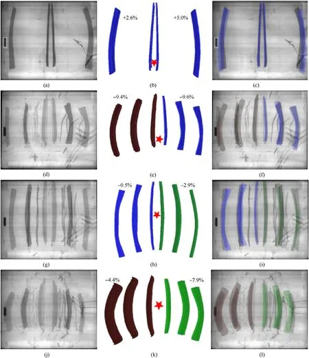
Fig.4.Validation of the numerical model with X-ray images;images are rotated by 90◦(left half first plate and right half second plate):(a)Experiment #1;(b)Simulation #1;(c)Comparison #1;(d)Experiment #2;(e)Simulation #2;(f)Comparison #2;(g)Experiment #3;(h)Simulation #3;(i)Comparison #3;(j)Experiment #4;(k)Simulation #4;(l)Comparison #4;Materials are indicated by different color:Mars®240(blue),AA 7020-T651(red),Ti6Al4V(green);the percentage difference of plate velocity in the simulation is denoted in black;the detonation point is indicated by a red star.

Fig.5 and Fig.6 comprise three studies:(i)the amount of simulations required,(ii)the refinement of the training data,and(iii)the network architecture.Each plot shows the root-mean-squared training loss for the training set(solid line)and the validation set(dashed line);10% of the simulations are validation data.

Regarding(i)(shown in Fig.5(a)),both losses-training and validation loss-decrease with more simulations used for training.It reaches a local minimum for 200 simulations and then stays at the same magnitude.Indeed,the case with 100 simulations results in a sufficiently small loss.However,comparing the qualitative behavior of 100 and 1000 simulations,differences are visible(compare Fig.5(b)),whereas the results of 1000 and 5000 simulations are almost the same(not depicted in the paper).Therefore,a conservative choice is to use 1000 simulations.However,if the generation of training data is more expensive,200 simulations give a good approximation,too.

Fig.6 shows the influence of the discretization on the loss.The coarser discretization selects a subset of equidistant sensors(spatial)and a reduced number of time steps(temporal).The discretization of the simulations stays the same.Already for a very coarse discretization in space and time,the loss is little.The influence from the time discretization seems almost negligible.This might be related to the fact that the shape does not change significantly over time and the magnitude is already well captured by a few time steps.However,it has to be noted that the validation loss is also evaluated at exactly the time steps that were used for training.At this point,it would be interesting to see how well a model with only 10 time steps can estimate intermediate time steps-in particular,during the beginning of the simulation.In this study the time steps for training were chosen equidistant;in the future,a random choice of time steps can be of interest.Regarding spatial discretization,the difference in the loss for a coarse resolution is more significant.Using about 30 sensors seems to be sufficient.Here,the visualization of the plate bending shows directly that the curves are so smooth that 30 sensors are sufficient to represent the bending.

Fig.5.Optimization of the ANN:influence of the number of simulations(i)Training and validation loss;(ii)Prediction with 100 simulations as input data shows differences to the ground truth;(iii)Prediction with 1000 simulations as input data matches well.(a)Convergence;(b)100 Simulations;(c)1000 Simulations.

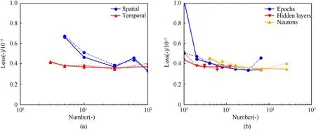
Fig.6.Optimization of the ANN:training and validation loss(i)for a reduced amount of training samples per simulation,and(ii)for different choices of architectures in terms of hidden layers and neurons,and the amount of epochs for convergence.(a)Discetization of the data;(b)Network architecture.

To optimize the network architecture,a simple ANN template is chosen as described in section 3:it contains an input layer,a certain amount of hidden layers with a constant number of neurons,and an output layer with one output(plate position of the configuration y(x,t)).The unknowns of this architecture are the number of neurons and hidden layers.Furthermore,it needs to be investigated how many epochs are required for the training.Fig.3 presents the results for these three properties of the ANN.For the number of hidden layers,one obtains already good results with only one layer.The approximation quality improves with a second and third layer;more layers do not give an additional benefit.Hence,three layers are used in the final model.A more significant amount of neurons improves the training loss.However,if too many neurons are used the validation error increases which is an indication of overfitting.Therefore,16 neurons are chosen as they seem to be an acceptable compromise between training loss,training time,and overfitting.The number of epochs is also investigated in this context,although it is not a part of the architecture.One epoch is not enough to train the model sufficiently well.There is a small benefit of using more than two epochs.Eight epochs seem to be a good trade-off between training time and training loss.For 32 epochs the validation loss increases similar as seen for 128 neurons.

In brief,this comprehensive study showed that 1000 simulations evaluated at 30 sensors and 10 times are sufficient for a small training loss.By this,the data set is reduced from 100.000.000 to 600.000 training samples.Regarding the network architecture,much fewer layers and neurons were needed than expected.In practice,the ANN consists of three hidden layers with 16 neurons each,and eight epochs are used in the final model.The training of this minimalist ANN takes about 1 min.

5.2.Comparison of the analytical model and the ANN with the numerical simulation

Fig.7 compares the ANN result with the numerical simulation(which is the ground truth of the ANN)and the analytical model by Chanteret for the four configurations tested in the experiment.As seen in section 4.1,the analytical model is well capable to predict the final plate velocity for all four tested configurations.However,it does not account for the acceleration phase that is important for an ERA.Due to the acceleration phase,the model of Chanteret is predicting a larger displacement of the plate in all cases.The ANN,on the other hand,does not only learn the correct velocity but also represents the acceleration phase and bending,which depends on the eight design parameters,acceptably well.Therefore,the ANN is a useful,easy-toapply methodology to predict the behavior of an ERA in real-time.

Fig.7.Comparison of numerical simulation(ground truth for the ANN),ANN prediction,and analytical model;the ANN is well capable to predict the shape and velocity of the plate;the analytical model only predicts the final plate velocity correctly(distance between t1 and t2 is correct,but value of t1 is too large)).

6.Outlook and discussion

An ANN was designed that predicts the kinematic behavior of an ERA with arbitrary plate size,plate thickness,material,and position of the detonation point.The network was successfully trained with data extracted from numerical simulations.Four example configurations were detonated in experiments to validate the numerical model.Except for spallation,which was not modeled,good accordance between the simulation and the experiment is found.Optimization of the ANN showed that 1000 simulations evaluated at 30 sensors for 10 times are required for the training.A shallow ANN with three hidden layers of 16 neurons each is sufficient to learn the regression problem.

Besides being the first step towards a pre-design of ERA configurations,this work showcases the simplicity of an ANN to solve this kind of regression.In comparison,a classical look-up table suffers under the curse of dimensionality;e.g.,four values for each of the seven design parameters already require 2400 simulations and give a coarse resolution of the parameter space.Higher-order interpolation does allow to evaluate configurations in the entire discretization space,too.However,this requires at least as much effort as implementing an ANN.

The network unveils the possibility to pre-design an ERA and to identify optimal designs.This project is part of ongoing work,further investigations will probably deal with optimized pre-design of an ERA for a set of different impact scenarios(projectile length,velocity,impact position,impact angle).

Declaration of competing interest

The authors declare that they have no known competing financial interests or personal relationships that could have appeared to influence the work reported in this paper.