Novel extended C-m models of flow stress for accurate mechanical and metallurgical calculations and comparison with traditional flow models

Man Soo Joun,Moh Kaswanee Razali,Jae Dong Yoo,Min Cheol Kim,Jeong Muk Choi

a ReCAFT,Gyeongsang National University,Graduate School of Mechanical and Aerospace Engineering,Jinju 52828,South Korea

b Gyeongsang National University,Graduate School of Mechanical and Aerospace Engineering,Jinju 52828,South Korea

c MFRC,Research Center,Jinju 52818,South Korea

d Jinhap,Daejeon 34302,South Korea

Abstract Here,we developed novel extended piecewise bilinear power law (C-m) models to describe flow stresses under broad ranges of strain,strain rate,and temperature for mechanical and metallurgical calculations during metal forming at elevated temperatures.The traditional C-m model is improved upon by formulating the material parameters C and m,defined at sample strains and temperatures as functions of the strain rate.The coefficients are described as a linear combination of the basis functions defined in piecewise patches of the sample strain and temperature domain.A comparison with traditional closed-form function flow models revealed that our approach using the extended piecewise bilinear C-m model is superior in terms of accuracy,ease of use,and adaptability;additionally,the extended C-m model was applicable to numerical analysis of mechanical,metallurgical,and microstructural problems.Moreover,metallurgy-related values can be calculated directly from the flow stress information.Although the proposed model was developed for materials at elevated temperatures,it can be applied over a broad temperature range.

Keywords: Flow stress;Power law model;Piecewise bilinear function;Numerical analysis;Microstructural prediction;Peak strain.

1.Introduction

The flow behavior of metallic materials at elevated temperatures can be quite complicated;however,predicting this behavior is essential for engineering applications involving mechanical and metallurgical processes.Advances in numerical simulation technologies have provided some insight;for example,models have demonstrated that the behavior of light metals,including aluminum and magnesium alloys,depends strongly on the alloy materials,the associated weight percentages,and the history of the manufacturing processes or pre-work.Flow behaviors of magnesium alloys such as AZ80,AZ90,and titanium alloy,Ti-6Al-4V,allow hot metal forming only over a narrow range of the state variables,e.g.,strain,strain rate,and temperature.In this context,the accuracy of the state variables is essential for successful process development based on simulation and/or optimization technologies[1–3];however,these variables are too complicated to be simply formulated in a mathematical form.Compared with steel and aluminum alloys,the fitted flow stress error for magnesium alloy is considerably larger [4].Additionally,when a material experiences dynamic strain aging [5–7],the flow behaviors become too complicated to be formulated in the traditional way.

There are several major types of flow behavior models,including the Arrhenius equation model,Ludwik model,Voce model,andC-mmodel,among others.All flow models are based metallurgically or phenomenologically on specific functions with a few constants,which can be applied only to a limited number of commercial metals under specific conditions.

The hyperbolic sine Arrhenius model presented by Sellars and McTegart [8] has been employed widely to characterize the flow behaviors of materials [9–32],as it offers several advantages.For example,it is based on the metallurgical background,and can be applied over a wide range of state variables with the exception of strain.However,it lacks practicality to some degree due to difficulties in finding the material constants and excluding strain effects.Strain effect compensation schemes utilize high-order polynomials (up to the 14th order for Al6061 [33]),along with many material constants that further complicate the flow stress calculations and introduce instability.This is not advantageous when the peak strain (εP) and strain at the stress reaching a half kinetic dynamic recrystallization (ε0.5) [34–36],etc.need to be calculated for metallurgical prediction,due to the high nonlinearity of the material parameters.

The Ludwik model,or power-law model,and variants thereof [9,10,37–44] have been used to simulate material flow behavior,as represented by the Fields–Bachofen equation.The material parameters,including the strength coefficient(SC),strain-hardening exponent (SHE),and strain rate sensitivity (SRS),are formulated as functions of the state variables of strain,strain rate,and temperature.For example,Sutton and Luo [9] formulate the SC and SRS as a function of temperature.El-Magd and Abouridouane [41] simulated the deformation and fracture behavior of lightweight alloys;however,the effect of strain rate on flow stress was not considered in their study.Cheng et al.[42] express the SC as a logarithmic function of the strain rate,while the SRS is formulated as a function of temperature.Takuda et al.[43] assume a temperature-dependent SC and SRS,whereas the SHE is represented in terms of the strain rate and temperature.Hadadzadeh and Wells [44] formulate the SRS as a function of the strain,temperature,and strain rate.

Various two-stage models [4,10,45–53],as exemplified by the Voce model,have been utilized for modeling complicated flow stresses,with an emphasis on dynamic recrystallization.Basically,this model type divides the flow stress into two parts: one part considers the earlier stages of work hardening and dynamic recovery and the other part focuses on the dynamic recrystallization regime.Voce-type models tend to have many parameters and constants that must be determined;thus,application tends to be complicated.

There are also many material models that do not belong to the major three aforementioned types.For example,Hadadzadeh and Wells [44] present a mixed model of hyperbolic sine Arrhenius and exponential equations for the four divided regimes of strain rate and temperature,to more accurately predict the flow behavior of ZK60 magnesium alloy.During the last decade,artificial neural network-based material characterization has also been applied [54–57],and excellent agreement between theoretical predictions and experimental results has been demonstrated.

Some researchers have concentrated on closed-form material models.However,it has been concluded that the constant material parameters applied in this model type are not appropriate for flow stresses locally representing dynamic recrystallization,and that a simpler approach is necessary for computer-aided engineering applications.An accurate description of the strain or strain rate softening at elevated temperatures is of great importance for improved engineering calculations,e.g.,the slope and magnitude,for example,corresponding to the peak strain and steady-state strain,respectively,to predict microstructural phenomena with higher accuracy.It is noteworthy that the number of material constants in the flow stress model is not a significant concern in this computer age,as most can be managed in numerical analyses.Additionally,the greater the number of material constants,the higher the accuracy and flexibility of the model.However,despite the remarkable dedication and efforts of researchers in this field for several decades,no such model has been developed.

The peak strain that governs microstructural evolution should be characterized independent of the flow stress,as most studies have focused mainly on the accuracy of the flow stresses.In addition,most studies concentrated on a specific metallic material and the associated accuracy of the characterization,as opposed to a more general construct.In this paper,a novel extended piecewise bilinearC-mmodel is presented,with an emphasis on its compatibility with other numerical approaches,as well as its generality and peak strain and stress prediction accuracy.

2.Representative flow stress models and a new material model

2.1.Arrhenius equation model

The Arrhenius flow stress model,and variants thereof,have been utilized to characterize metallic alloys,as presented by Sellars and McTegart [8] as follows:

The original Arrhenius equation cannot deal with the effect of strain on the flow stress.This problem was solved by the strain compensation scheme,which formulates the material parameters as a function of strain.Most researchers used high-order polynomials.For example,Sutton and Luo [9],Dong et al.[10],Luan et al.[12],Changizian et al.[32],and Rudnytskyj [33] characterized as-cast AZ81,as-extruded AZ31,commercial AZ31,commercial ZE20,and Al6061 using polynomials of order 4,5,6,8,and 14,respectively.It should be noted that the increased polynomial orders showed some oscillatory values at higher strains,as discussed by Lin et al.[58],which reduced the reliability and generality of the scheme.The use of higher order polynomials makes it difficult to calculate the secondary values necessary for prediction of microstructural evolution directly from the flow stress information,including the peak and steady-state strain.

All of the parameters of the modified hyperbolic sine Arrhenius equation,includingα,n,Q,and ln(A),can be described by the following strain polynomial:

whereNranges from 4 to 14 in the literature,and the constantsCiare determined by minimizing the error between the experimental and fitted flow stresses.

2.2.Ludwik model family

Several flow stress models can be classified as extended Ludwik models,the mechanism of which is stated asσ=Y0+Y1εn.The two constants,and the exponent,in the extended formulation can be expressed as functions of strain rate and temperature (or can be assumed to have a value of zero).Basically,the flow stress dependences on the strain rate and temperature in these models are dealt with by multiplying separable functions of the strain rate and temperature.

The Johnson–Cook model [59],a typical Ludwik model,employs the fewest material constants.Due to its simplicity,the Johnson–Cook model is widely used in engineering,although it is beneficial mostly for large strain rate problems;it may not provide acceptable predictions for non-isothermal analysis of metal-forming processes of metallic materials that exhibit complicated flow behaviors.Other well-known Ludwik models include the Khan–Huang–Liang flow stress model[60,61].However,most traditional Ludwik models cannot readily be applied to solve practical engineering problems related to metal forming,in which complicated dynamic recrystallization occurs;however,they can accommodate mechanical applications involving high strain rate deformation under impact,explosive forming,and crash conditions.

Sutton and Luo [9] presented an extended Ludwik model starting from the following traditional strain and strain rate hardening model:

whereK[MPa],n,andmare the SC,SHE,and SRS,respectively,andis a reference strain rate,assumed to be 1/s in this study.Eq.(3) is known as the Fields–Bachofen equation model [62].Assumingdln(σ)/dεis a linear function ofeBε,whereBis a constant,they formulated the SHEnas follows:

The material parametersm,K,A,B,C,andDwere formulated as

wherem0,m1,K0,K1andCi’s are material constants determined such that they minimize the error between the experimental and fitted flow stresses.

Similar to the approach of Sutton and Luo [9],this kind of extended Ludwik model can be utilized for metal forming applications only when the parameters are formulated by high-order polynomials and/or specifically constructed functions,which could potentially negate the original benefit of this approach.Such an involved mathematical formulation to extract the material constants severely undermines the generality,which is important for practical application.

The Hensel–Spittel model (H-S) [63] can also be included in this family of models;its formulation,with nine material constants,is as follows:

where allmivalues are material constants.

Note that the H-S model is essentially a combination of the classical power law model of the strain rate and Hollomon and Swift models,having material constants considered as functions of strain and temperature.Basically,all of the nine material constants are constant;thus,Eq.(8) describes the flow behaviors over all of state variables with nine material constants.However,inaccuracies are inevitable in many cases,especially in expressions of strain softening behaviors,owing to the dynamic recrystallization.

2.3.Voce model family

Voce [64] represents flow stress as a function of strain,strain rate,and temperature,with an emphasis on microstructural evolution,as follows:

whereXdynis the volume fraction of dynamic recrystallization,defined as

whereσo,σP,σS,εP,andεsare the initial yield stress,peak stress,steady-state stress,peak strain,and steady-state strain,respectively,and are formulated by the Zener–Hollomon parameterZwith many material parameters or constants [8].

This model has many advantages.For example,the strain hardening effect,which should be dominant for strains smaller than the peak strain,decays very quickly as the strain increases,compatible with actual hot forming of commercial metals.This model can also accommodate typical strain softening owing to dynamic recrystallization.Unfortunately,it has some difficulties in identifying material constants or parameters;thus,it has few applications,despite being based on metallurgical theory.Considering this difficulty,practical approaches based on phenomenological models with fewer material constants have been developed.

Fig.1.Piecewise bilinear expression of material constants using the sample grid points in the form of φ (strain,temperature).

The model developed by Ebrahimi et al.[65] can be classified as a Voce model,although its background differs considerably from the Voce model.The Ebrahimi et al.model is fully phenomenological,whereas the Voce model tends towards a more physical model.However,they can both describe dynamic recrystallization.

The model of Ebrahimi et al.is given by

whereCsandCsare material parameters or constants.Ebrahimi et al.[65] derived a general systematic scheme using experimental plots showing the relationships between variables and/or parameters,not only to calculateChandCsbut also to formulateεp,σpandσSas functions of strain rate and temperature as follows:

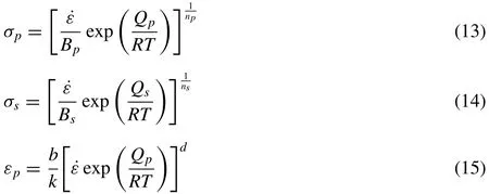
whereBp,Qp[kJ/mol],np,Bs,Qs[kJ/mol],ns,b,kanddare the material parameters that obtained through the graphical approach.The scheme assumes that the experimental plots are linear.The fitted linear functions are used to interrelate variables and/or parameters to identify flow stresses at particular strains,strain rates,and temperatures.

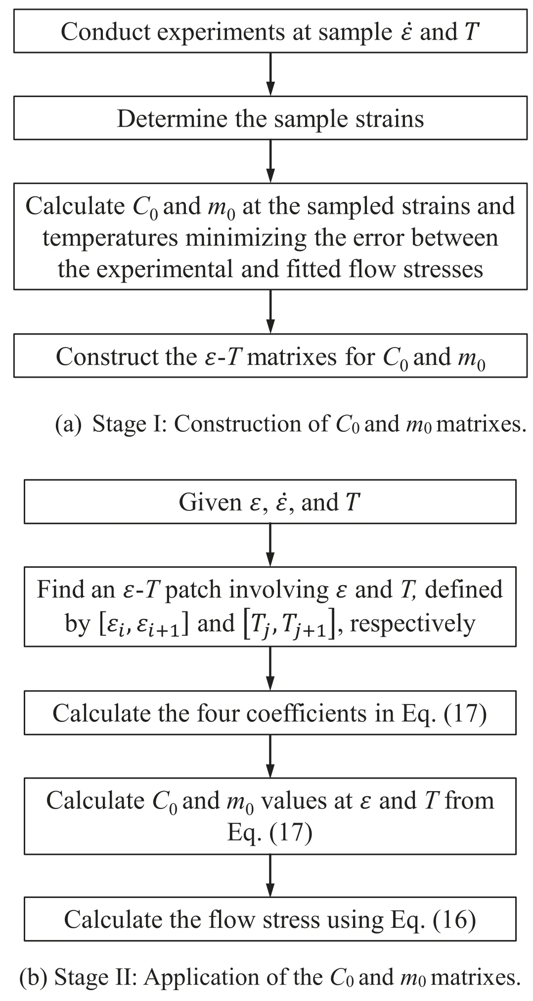
Fig.2.Flowchart of constructing the flow database and calculating the flow stresses.

Razali et al.[4] developed a systematic formulation and identification scheme of describing material parameters includingCh,Cs,εp,σpandσSusing piecewise bilinear functions of strain rate and temperature (i.e.,the PLF model.See Section 2.4),which can be applied regardless of the dependence on state variables.They applied their scheme successfully to commercial steel 20MoCrS4,aluminum alloy AHS-2,and magnesium alloy AZ80.

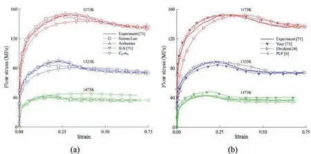
Fig.3.Comparison of fitted flow stress curves with the experimental flow stress of 20MoCrS4 at 0.1/s: (a) Sutton–Luo,Arrhenius,H–S and C0–m0 models and (b) Voce,Ebrahimi and PLF models.

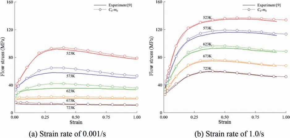
Fig.4.Comparison of fitted flow stress curves with the experimental flow stress of ZE20.

Fereshteh-Saniee et al.[46,47] characterized the flow behavior of various magnesium alloys,including AZ31,AZ80,and AZ81,using the Ebrahimi et al.model,in which the material constants were determined graphically.The graphical approach is inherently poor in terms of practicability and computerization.It hinders the formulation of material constants and parameters as functions of state variables including strain,strain rate,and temperature,which is essential to describe complicated flow behaviors with higher accuracy.To overcome this,Razali et al.[4] suggested a systematic scheme for calculating the material parameters as functions of state variables,using material constants that can be determined by optimization techniques;Razali et al.applied this scheme to the Ebrahimi et al.model for the magnesium alloy,AZ80,studied by Fereshteh-Saniee et al.[46,47].They compared their scheme with the original Ebrahimi et al.graphical approach to emphasize the advantage of the former.However,their method also requires additional effort to identify the optimal material constants,thus limiting computer-aided functionality and general usage.Overall,this type of model is limited in its ability to describe the peak strain and stress as functions of state variables,as demonstrated by Zeng et al.[53] for GW83 alloy,AZ31B,and ZK61,thus reducing the practicability of these flow behavior models.

Other flow behavior models include those of Xu et al.[48] for Fe-Mn-Al steel,Bergström [49] forα-Fe,Laasraoui and Jonas [50,51] for four low carbon steels,Serajzadeh and Taheri [52] for high-and low-carbon steels,and Qin et al.[45] for ZK60.

2.4.Traditional piecewise bilinear C-m model

The most common and general flow stress model for the material at elevated temperature is the following traditionalC-mmodel,i.e.,the power-law model:

whereC0[MPa] is the strength parameter andm0is the SRS.Eq.(16) shows the conventional form.C0andm0are commonly considered as constants,especially in isothermal analyses.In non-isothermal analyses,C0andm0have traditionally been modeled as piecewise bilinear functions of the strain and temperature as follows:

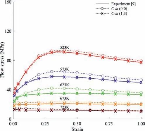
Fig.5.Fitted curves for the C-m (1:3) model.

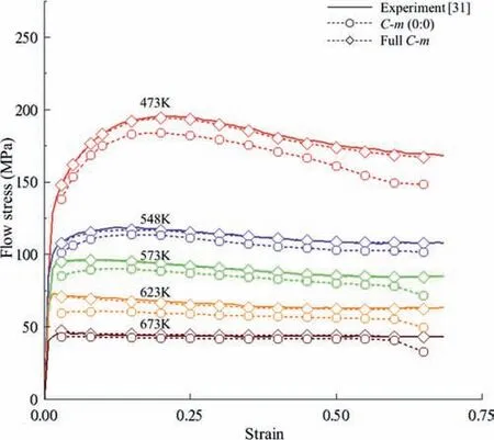
Fig.6.Comparison between full C-m and C0-m0 models at a strain rate of 0.1/s.

WhenC0andm0are described piecewise on a rectangular mesh of strain and temperature,as shown in Fig.1,their values at an arbitrary point A*(ε,T) inside a patch,represented byφ(ε,T),can be bilinearly interpolated by Eq.(16) with the known nodal values ofC0andm0,denoted byφi(i=1,2,3,4) and defined at the grid points:

Fig.2 shows the flow charts of the schemes of constructing the flow database and calculating the flow stresses using Eqs.(16) and (17).The nodal valuesC0andm0at each grid point,in which the temperature and strain are fixed,can be calculated using an optimization technique.C0iandm0irepresent the flow behaviors at a fixed temperatureTiand fixed strainεi;they are thus calculated by the optimally fitting scheme in the stress–strain rate domain.Notably,the calculations and procedure can be automated easily,as can be easily recognized in Fig.2(b).WhenC0andm0are described by constants,as given above,theC-mmodel is then referred to specifically as theC0-m0flow model.

The above scheme is readily applicable to numerical analyses.In contrast,the flow stress described using Eqs.(16)and(17) is not appropriate ifC0andm0are constant (i.e.,do not change monotonically with respect to the strain rate at the sample strain and temperature).In addition,as revealed in the case of an aluminum alloy by Park et al.[66],the traditionalC-mmodel,i.e.,theC0-m0model,inevitably includes some error,due to the complicated relationship between the SRS and strain rate.According to Malik et al.[31],the dependence of the SRS on the strain rate itself can be significant.For example,given a fixed strain and temperature of 0.1 and 673 K,respectively,the SRS ranged from around 0.14 to 0.42.

There are two major shortcomings associated with theC0-m0model.First,it has some difficulty in representing the negative SRS.In other words,the model is insufficient when for describing flow stress behaviors exhibiting strain rate softening.Notably,these behaviors are of great importance for detecting plastic deformation instability during the hot forming of difficult-to-form materials,including aluminum and magnesium alloys.Second,this model cannot be used to obtain the processing map developed by Prasad et al.[67–69],because the SRS is constant when the strain and temperature are fixed.It should be noted that these two factors are magnified in materials with bad formability,such as in aluminum and magnesium alloys that exhibit some form of plastic deformation instability.

2.5.Discussion

We fitted flow stress curves of the steel 20MoCrS4 presented by Meyer et al.[70].Note that 20MoCrS4 (chemical composition in wt%: C 0.20;Si 0.25;Mn 0.75;Cr 0.40;Mo 0.45;S 0.02;Pb to 100 wt%) exhibits typical strain softening owing to dynamic recrystallization.Additionally,they characterized the material using two sample strain rates of 0.1 and 10/s at three sample temperatures: 1173,1373,and 1,473 K[70].

Fig.3 compares the experimental data of a hot cylinder compression test of steel at a strain rate of 0.1/s with curves fitted by the H-S [63],Voce [64],Arrhenius [8],Sutton–Luo[9],Ebrahimi et al.[65],and PLF [4] models,as well as theC0-m0flow model.The H-S and Voce fittings were reported by Meyer et al.and Ebrahimi et al.,and PLF fittings were made by Razali et al.[4].The material constants of the newly calculated flow models are summarized in Table 1.

Table 1 Material constants of the models newly applied.

Table 2 Maximum and average errors of different models used to evaluate 20MoCrS4 at a strain rate of 0.1/s.

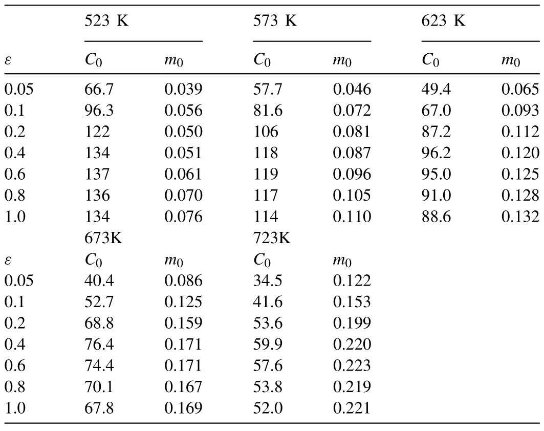
Table 3 Material constants for C0-m0 model used to evaluate ZE20.

Table 4 Maximum and average errors of C0-m0 models used to evaluate ZE20.

Table 5 Evaluation of the selected C-m models.

Table 6 Material constants for C-m (1:3) model of ZE20.

Fig.7.Comparison of fitted flow stress curves with the experimental flow stress of the ZK61.

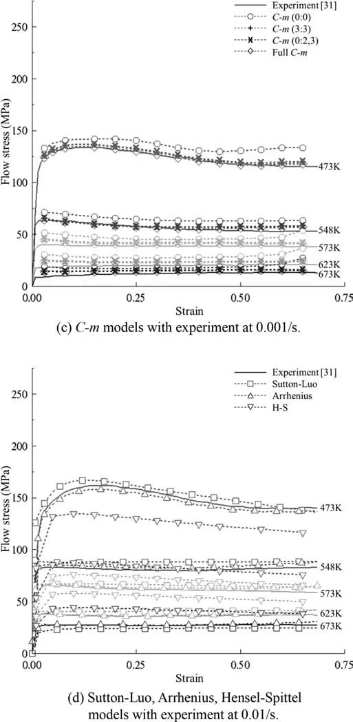
Fig.7.Continued

Fig.7.Continued

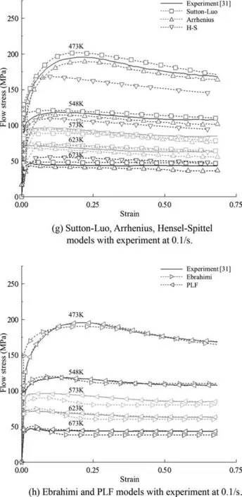
Fig.7.Continued

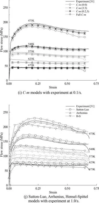
Fig.7.Continued

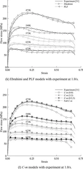
Fig.7.Continued

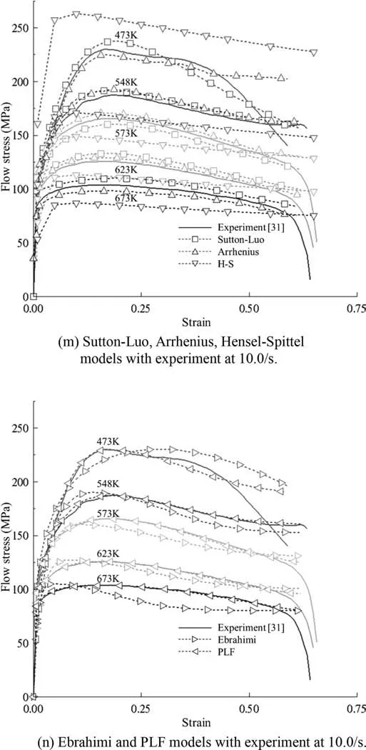
Fig.7.Continued

Fig.7.Continued

From Fig.3,theC0-m0flow model well fit the experimental results,because two sample strain rates were applied to determine two unknown material constants at the grid point of sample strain and temperature.Fig.3 also shows that the PLF model and hyperbolic sine Arrhenius equation model(sixth-order polynomial) well fit the experiments;moreover,their extremum points coincided with those of the experiments.However,the models of Johnson–Cook,H-S,Sutton–Luo,and Ebrahimi et al.exhibited large errors for both the flow stress and peak strain.Conversely,the Voce model predicted flow stress with acceptable accuracy,and was fairly accurate in predicting peak strain.

Table 2 compares the flow stress models quantitatively.The maximum and average errors of theC0-m0flow model were zero.Although these results were obtained based only on the two strain rate cases in the example,they are sufficient to show the characteristics and advantages of theC0-m0model.

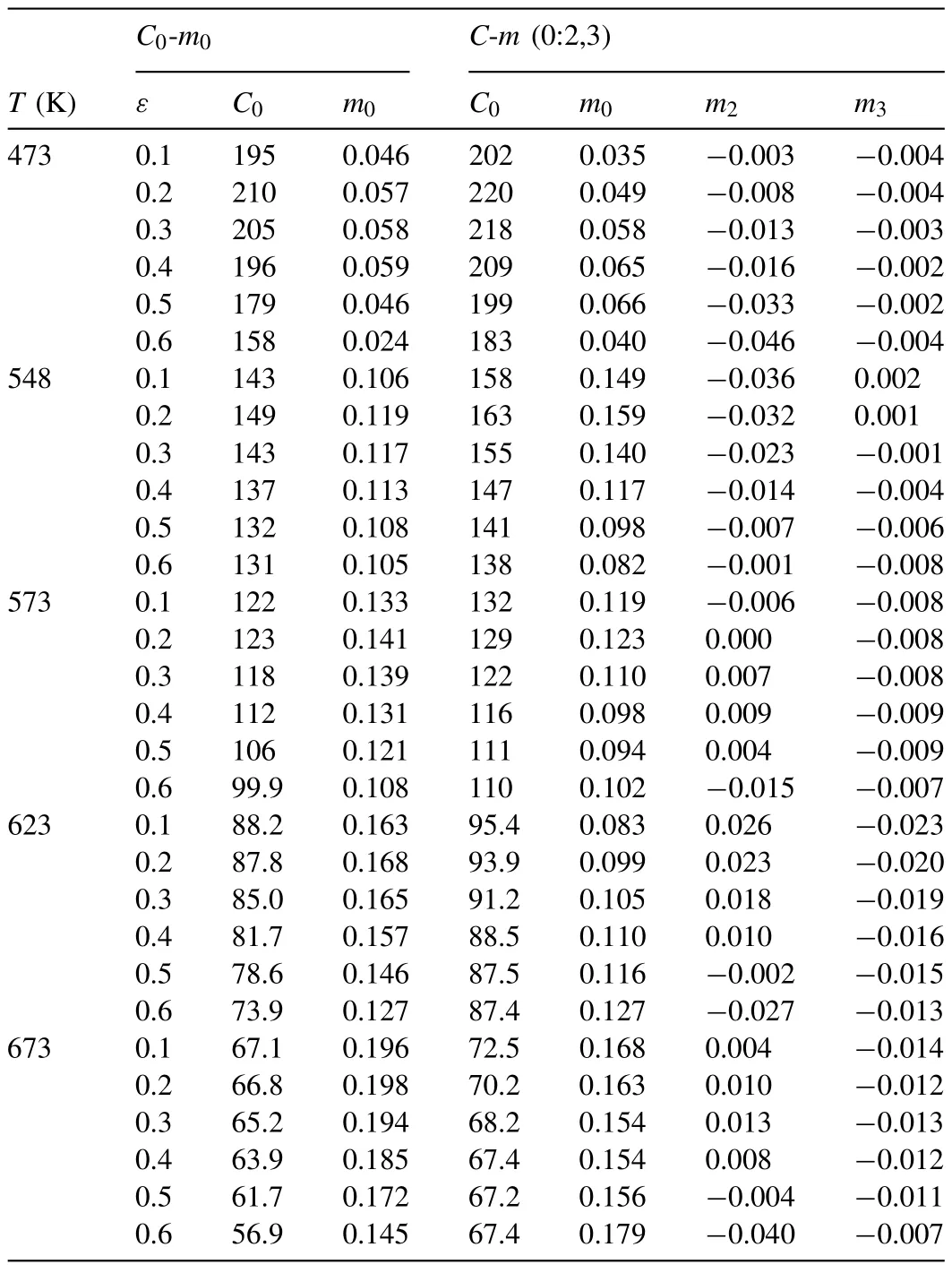
Table 7 Material constants of C0-m0 and C-m (0:2,3) models.

Table 8 Error evaluation of the selected C-m models.

The maximum and average errors at the sample temperature of the PLF (5.17% and 2.09%,respectively) and Arrhenius (7.03% and 2.31%) models were less than those of Sutton–Luo (7.81% and 4.01%),Ebrahimi et al.(14.60%and 4.75%),Voce (17.08% and 12.88%),and H-S (20.82%and 14.02%) models.Based on the average error,we can order the flow stress models in this example as follows:

C0-m0>PLF,Arrhenius>Sutton-Luo

Now it is by no means certain that ‘Donkey Skin ‘ had not caught a glimpse of the prince, either when his eyes looked through the keyhole, or else from her little window, which was over the road. But whether she had actually seen him or only heard him spoken of, directly she received the queen’s command, she flung off the dirty skin, washed herself from head to foot, and put on a skirt and bodice of shining silver. Then, locking herself into her room, she took the richest cream, the finest flour, and the freshest eggs on the farm, and set about making her cake.

>Ebrahimi et al.>Voce>H-S

Consequently,the higher order polynomials for the Arrhenius model and piecewise bilinear expressions of the material constants and parameters of theC0–m0and PLF models gave good approximations of both the flow stress and peak strain.Of course,the other flow models are also able to provide more accurate fittings if they employ such schemes at the expense of some practicability.It should be emphasized that the accuracy of peak strain was better for theC0–m0,PLF,Arrhenius,and Voce models,which is important in metallurgical calculations.Moreover,the PLF model can be employed to calculate microstructural evolution,without any additional formulation ofεPandε0.5[71];in this context,Voce models offer some advantages for metallurgical purposes when accurately expressed.

The key problems concern practicability,computerizability,and reliability.In this regard,the piecewise bilinearC0–m0flow model is promising,not only because it can easily be computerized for high applicability but also because its material constants are easy to handle,as they do not require non-linear order terms for the strain.The piecewise expression of the function of strain and temperature can be expressed with high versatility using a set of sample points of the strain–temperature mesh [form: (strain,temperature)]shown in Fig.1.Therefore,the material constants of the piecewise bilinearC-mmodel do not have to involve any strain or temperature terms [7].

However,theC0-m0flow model can predict the fitting at the sample points only when the sampled experimental strain rate is one or two,although there is no limitation on the number of sample points of strain and temperature.That explains why the fitted curves are exact in this example.Therefore,one of the drawbacks of theC0-m0model is that accuracy is dependent mainly on the two material constants at the grid points.The increase in numbers of sample strains and temperatures does not have a significant effect on the accuracy.

3.Extended piecewise bilinear C-m model

In the previous section,the advantages and characteristics of the traditional piecewise bilinearC0-m0model were explained.Its drawbacks,however,were not quantified.We thus applied the approach to four sample strain rates to evaluate theC0-m0model.

Sutton and Luo [9] conducted uniaxial cylinder compression tests of ZE20 billets at four sample strain rates,0.001,0.01,0.1,and 1.0/s,and at five sample temperatures,523,573,623,673,and 723 K,using a Gleeble 3800 servo-hydraulic thermomechanical testing system.

We performed the experiments using theC0-m0models;the material constants are given in Table 3.We selected two strain rate cases,that is,the maximum (0.001/s) and minimum (1.0/s) error cases of the fitted flow stress,shown in Fig.4(a) and (b),respectively.The maximum and average errors are summarized in Table 4,indicating that the maximum error of 20% occurred for a strain rate of 0.001/s and temperature of 623 K,whereas the minimum average error over all temperatures corresponded to a strain rate of 4.9%.Although the fitted peak strains (0.4) were nearly the same as those obtained experimentally (0.398),and the minimum average error of the case shown in Fig.4(b) is acceptable,the maximum error cannot be neglected.

It should be noted that the constant values ofCandm,similar to theC0-m0model,cannot describe the simultaneous strain rate hardening and softening phenomena for a fixed strain and temperature,which are of great importance for determining the metallurgical instability [7,67] of the materials during metal forming.

However,we find from Fig.4 that the fitted peak strains are almost the same as the experimental results,regardless of the accuracy of the flow stress,implying that the simpleC0-m0model can accommodate microstructural evolution predictions[71].

On the contrary,the simple model of Eq.(16) can even describe strain rate softening behavior when we formulateCandmas functions of strain rate at a fixed strain and temperature,as follows:

whereCi[MPa],miandγirepresent all material properties defined at the fixed sample strains and temperatures,similar toCandmin Eq.(16).They can be treated either as just constants or as piecewise bilinear functions of strain and temperature.They are calculated by minimizing the error between experimental and fitted flow stress functions.Some of them can be considered as fixed during curve fitting.With these extended functions ofCandm,all of the aforementioned problems of theC0-m0model were solved.All of the new material constants can be treated in the same way as the constantsC0andm0of theC0-m0model.

Eq.(18) appears to be very flexible in terms of the strain rate.Notably,this function is much more flexible with respect to the strain and temperature,because the functions are defined in a piecewise manner,as shown in Fig.1.The basic approach for calculating the material constants at the sample point is the same as the conventional scheme,and can be easily programmed and computerized.

Note that we called theC-m (i,j..:I,J..)model in the case whereC|i|=C|j|=..=non-zeros andm|I|=m|J|=..=nonzeros.The other constants,exceptC0andm0,should all be zero.C0andm0are all non-zero in any model;the index of zero can be deleted,andγican be considered as either fixed or variable.In the case that the index is -2,its corresponding constantγiis a variable that needs to be optimally determined.Otherwise,γihas a given value.Examples include theC-m(1:1) model in the case ofC2=C3=m2=m3=0,theC-m(1,2:2,3) model in the case ofC3=0 and m1=0,theC-m(3:3) model in the case ofC1=C2=0 andm1=m2=0,and theC-m(0:-2) model in the case ofC1=C2=C3=0 andm1=m3=0 (γ2is unknown),etc.TheC0-m0model can thus be described as theC-m(0:0) orC-m(:) model.We define the fullC-mmodel,which considers all of the constants as unknown variables.

We analyzed the characteristics of variousC-mmodels with four unknown constants at the sample strain and temperature in terms of both the average absolute relative error(AARE) and root mean square error (RMSE) using the same experiments.A set of fitted curves of theC-m(1:3) model that best fit the experiments are shown in Fig.5,indicating that the error cannot be meaningful,although the error ofCm(0:0) is significant.The analyzed results are summarized in Table 5,revealing that any combination of non-zero constants(Table 6)provided better fittings compared to theC0-m0model,and that the linear term for the SC is influential in the case of a very low strain rate (0.001,0.01,0.1,or 1.0).To the contrary,the logarithmic term was the most influential in terms of the SRS.Note that care should be taken when the linear terms for the material constants are applied in the wide and high strain rate case,wherein strain rate extrapolation is needed.

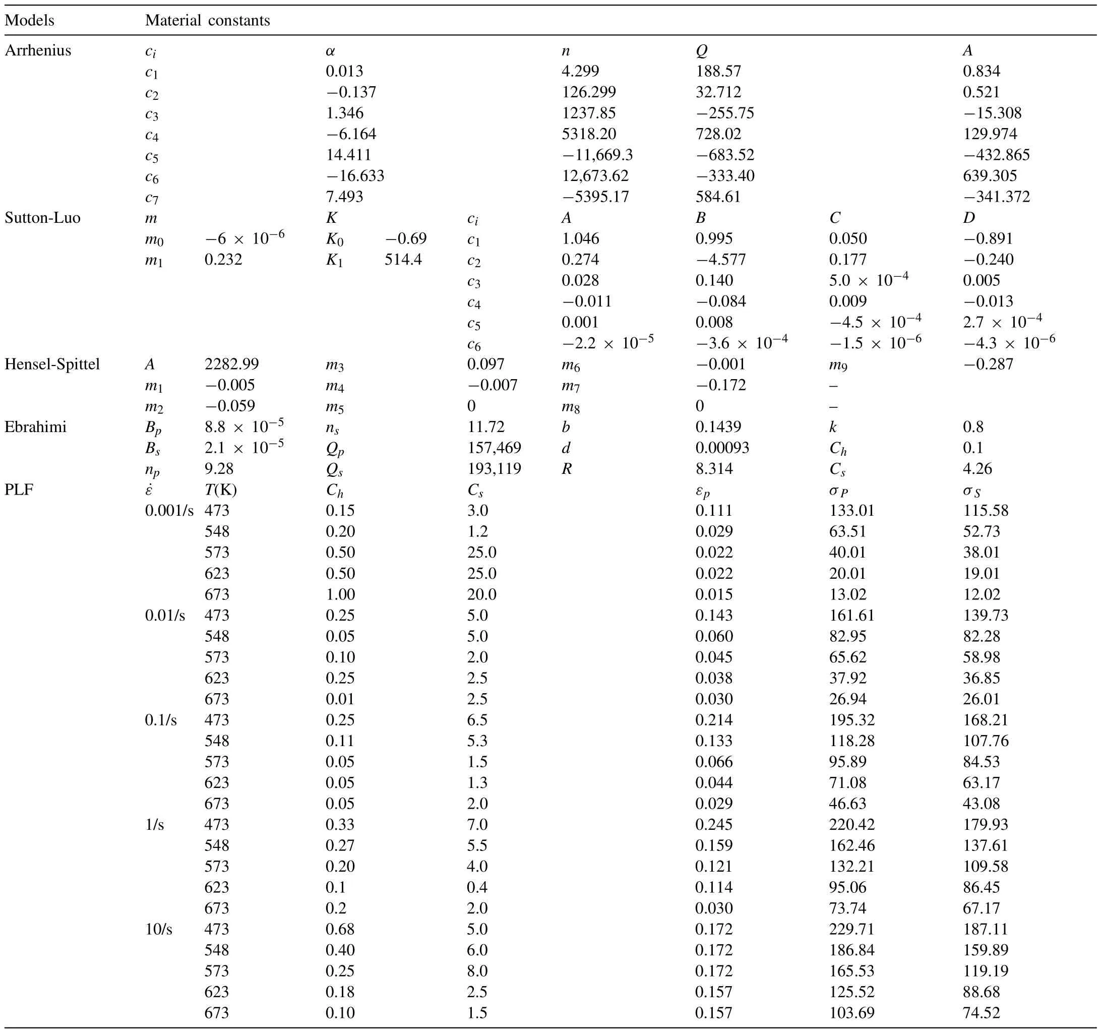
Table 9 Material constants of all closed-form function flow models applied to the ZK61.

4.Application of a new model to ZK61

Malik et al.[31] conducted a cylinder compression test of the commercially available extruded ZK61 magnesium alloy over a wide range of temperatures (298–673 K) and strain rates (0.001–10/s).Their experimental data are described bythe solid lines in Figs.6 and 7.It should be emphasized that the experimental data cover a relatively large range of strain rates (0.00–10/s),from among which five test strain rates (0.001,0.01,0.1,1 and 10/s) were selected.Thus,the flow stress curves are more complicated than in the two test cases in the previous sections.

We obtained the best-fitted flow stress curves using the fullC-mmodel,as shown in Fig.6,for the sample strain rate of 0.1/s.The fullC-mmodel was also compared with experiments and theC0-m0model,as shown in Fig.6;the results showed that the fullC-mmodel had an exact fit,whereas the traditionalC0-m0model exhibited significant error.

We conducted a detailed investigation into some of the selectedC-mmodels,including theC-m(0:0),C-m(1:1),Cm(1,2:0),C-m(0:1,2),C-m(1:2),C-m(2:1),C-m(1,3:0),C-m(0:1,3),C-m(1:3),C-m(3:1),C-m(2,3:0),C-m(0:2,3),C-m(2:3),C-m(3:2),andC-m(3:3) models.The detailed material constants of theC0-m0andC-m(0:2,3) models are given as examples in Table 7.Note that theC-m(0:2,3)model had minimal AARE and RMSE errors in the error analyses of the test models,as shown in Table 8.Table 8 indicates that all of the cases of theC-mmodel improved the fitted flow stress compared with the traditionalC0-m0model.Among the testC-mmodels with only four unknown constants,theC-m(0:2,3) model (γ2=0.5) was the best in terms of its AARE and RMSE values,which were 1.27% and 0.84 MPa,respectively.Conversely,theC-m(3:3) model was the worst in terms of both AARE and RMSE.However,Table 8 shows that the differences in AARE and RMSE between the best and worst trialC-mmodels were negligible,at 0.64% and 0.49 MPa,respectively;thus,the scheme is stable and strongly dependent on the number of unknown material constants in cases in which the strain rate is bound.

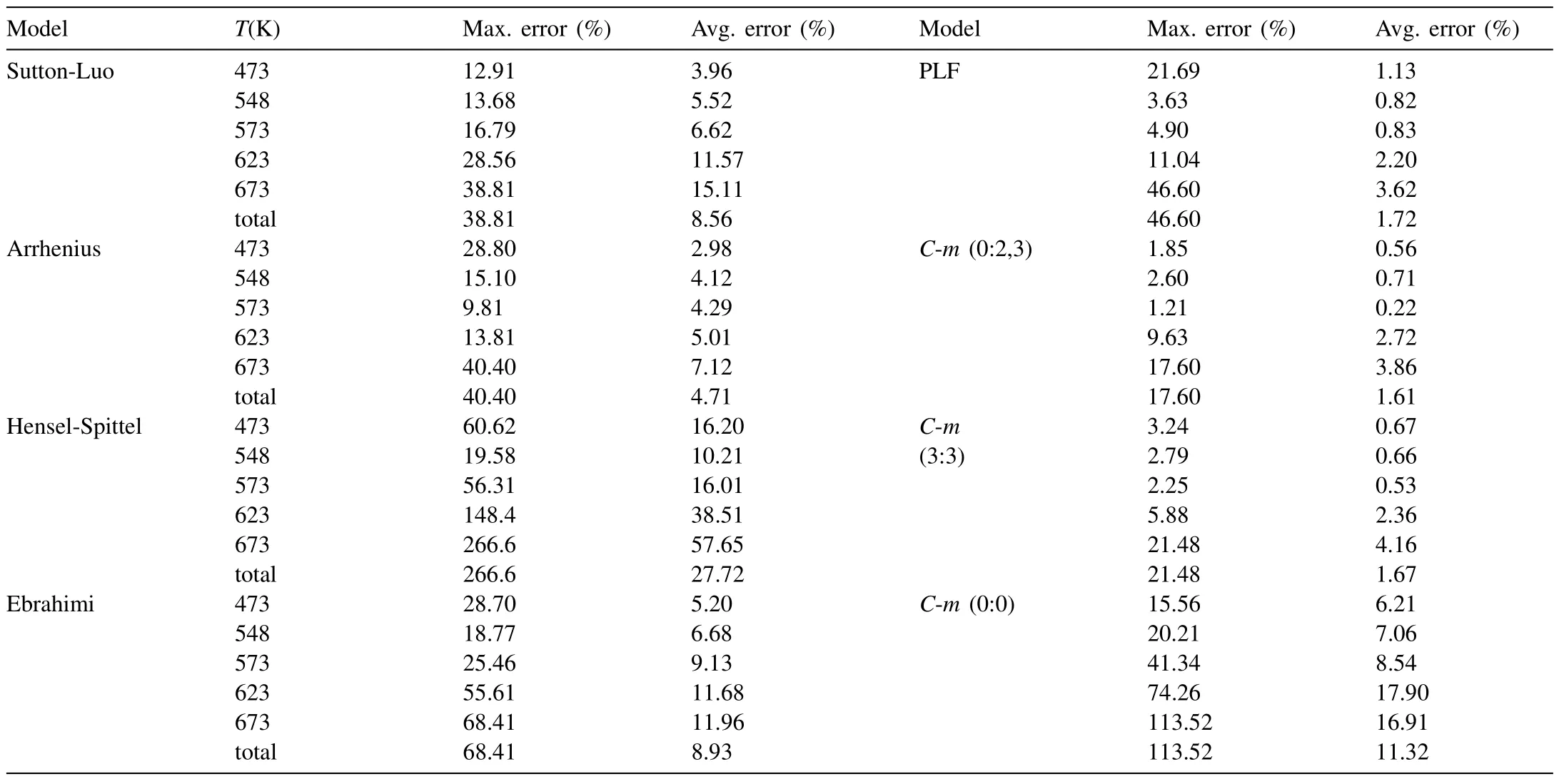
Table 10 Maximum and average errors of different models used to evaluate ZK61.

To evaluate the fitted flow stress curves of the extendedC-mmodel,we experimentally compared theC-m(0:2,3)model (γ2=0.4),C-m(3:3) model,andC-m(0:0) model[31].They were also compared with other models,including the hyperbolic sine Arrhenius model,Sutton–Luo model,HS model,Ebrahimi et al.model,and PLF model.TheC-m(3:3) model performed the worst among the testedC-mmodels,with the exception of theC-m(0:0) model,as shown in Table 8.We used the sixth-order polynomial of strain for the material parameters of the hyperbolic sine Arrhenius model.

The fitted material constants of all of the closed-form function flow models are summarized in Table 9.The models are compared in Fig.7,and the maximum and average errors over the ranges of strain (0.03–0.65) and temperature (473–673 K) are listed in Table 10.It can be seen thatC-m(0:2,3)is the best in terms of both the maximum(17.6%)and average(1.6%) errors.TheC-m(0:0) model exhibited the worst maximum (113.5%) and average (11.3%) errors among the testC-mmodels,while the H-S model showed the worst maximum and average errors,of 266.6% and 27.7% among all the test models,respectively.Of course,the maximum and average errors were exaggerated due to the small absolute values of the flow stresses at high temperature and low strain,as can be seen in Fig.7.Nonetheless,the comparison of the maximum and average errors in Table 10 provide some insight into the accuracy of the test flow models in terms of complicated flow behaviors.Acceptable average error was seen among the PLF,Sutton–Luo,and Arrhenius closed-form function models with material parameters,even though the maximum error at low temperature was significant.The worstC-mmodel,described by four unknown material constants,was nearly the same as the best case in terms of the maximum and average errors,implying that the extendedC-mmodel is mathematically stable.

The typical flow curves in Fig.7(a)–(l) at a low temperature of 473 K and low strain rate (0.001–1.0/s) exhibit dynamic recrystallization and are well described by all of the test flow models,with the exception of the H-S flow model.They were best fitted by the PLF,C-m(0:2,3),andC-m(3:3)models in terms of average and maximum errors,as listed in Table 10.Note that the error of each model in Table 10 was calculated at the 15 selected sample strains of 0.03,0.05,0.08,0.10,0.15,0.2,0.25,0.3,0.35,0.4,0.45,0.5,0.55,0.6 and 0.65.The flow behavior,especially at the temperature of 473 K and strain rate of 10/s shown in Fig.7(m) and (n),could not be properly expressed by the closed-form function models,so were described using the Sutton–Luo model.As summarized in Table 11,the maximum errors of the fitted curves of the closed-form function models at a strain of 0.55 are all greater than 21.7%,with the exception of the Sutton–Luo model.The drastic drop in flow stresses at the sample temperatures of 573,623,and 673 K could be described only by theC-m(0:2,3) andC-m(3:3) models,as shown in Fig.7(o).

Table 11 Maximum and average errors of different models at strain rate 10/s.

We compared the peak strains of the fitted flow curves at 473 K;at this temperature,the value could be clearly determined due to distinct dynamic recrystallization.The fitted peak strains,i.e.,those at the maximum flow stress point shown in Fig.7,were acceptable for theC-m(0:2,3),C-m(3:3),and PLF models,whereas the other flow models exhibited considerable differences from the experimental results at some of the sample strain rates.For example,the Sutton–Luo(0.001,0.01/s),Arrhenius(0.001/s),H-S(all sample strain rates),Ebrahimi et al.(0.001,10.0/s),andC-m(0:0) (0.001,0.1,and 1.0/s) models,at the strain rates shown in their associated brackets,had larger error in terms of the peak strains.

5.Conclusion

In this paper,we presented a novel extendedC-mmodel describing complicated flow stresses involving strain softening due to dynamic recrystallization,after reviewing representative flow stress models and classifying them as Ludwik/Hollomon/Swift,Voce,hyperbolic sine Arrhenius,orC-mmodels based on their fundamentals.All of the examined flow models,and the experiments on 20MnCrS4,which exhibited typical dynamic recrystallization,were compared with an emphasis on the hitherto unrevealed advantages of the traditional piecewise bilinearC-mmodel.

We presented a novel extended piecewise bilinearC-mmodel,in which the material parameters defined at various sample strains and temperatures are expressed by a linear combination of a constant and several functions of the strain rate with unknown constants;these constants are optimized using the least-squares method.Note that the piecewise bilinear model of flow stress,according to values defined at the grid point of a structured strain–temperature mesh,is very versatile in terms of the strain and temperature.The presented models were examined using the experimental flow stresses for ZE20 alloy,measured at the four test strain rates.The four unknown parameter cases are practical for describing the flow stress in numerical simulations of mechanical and metallurgical problems in metal forming.With theC-mmodel,we can calculate any state variable meeting certain requirements based on its derivatives,as well as the flow stresses,using a simple arithmetic scheme.

The new models were applied to ZK61,which exhibits complicated flow stresses at five sample strain rates ranging from 0.001 to 10/s.VariousC-mmodels were compared with the Johnson–Cook,Sutton–Luo,and H-S Ludwik models,the graphical Ebrahimi et al.[65] and PLF Voce models,and the hyperbolic sine Arrhenius model in terms of flow stress and peak strain.The testC-mmodels includedC-m(0:0) models with two unknowns at a grid:C-m(1:1),C-m(1,2:0),C-m(0:1,2),C-m(1:2),C-m(2:1),C-m(1,3:0),C-m(0:1,3),C-m(1:3),C-m(3:1),C-m(2,3:0),C-m(0:2,3),C-m(2:3),C-m(3:2);C-m(3:3) models with four unknowns at a grid;and the fullC-mmodel with six unknowns.

The fullC-mmodel fit the flow curves almost exactly over the entire ranges of the state variables of interest,whereas theC-m(0:0) model showed some inaccuracies,especially at higher temperatures at which flow behaviors are abnormal or complicated.This implies that the traditionalC-mmodel,i.e.,theC-m(0:0) model,is not appropriate for metallurgical prediction.From a practical standpoint,the four unknown variable cases can be recommended,as they were numerically stable and showed acceptable accuracy for both the flow stress and peak strain.The best and worst of these four cases did not show a remarkable difference in terms of flow stress or peak strain.However,care should be taken when the linear term is employed if extrapolation for a considerably large strain rate is inevitable,e.g.,for simulating crash or impact phenomena.

This extendedC-mmodel can be readily adapted to meet the accuracy requirements for estimating metallurgical quantities,as well as the flow stress.Additionally,the limitation of the traditionalC-mmodel with respect to calculating the processing map can be eliminated.It is thus concluded that the extended piecewise bilinearC-mmodel is superior for both mechanical (flow stress) and metallurgical (e.g.,peak strain)calculations to all material models examined in this study,even though the hyperbolic sine Arrhenius with higher-order polynomials,Sutton–Luo,and PLF models exhibited acceptable accuracy in terms of flow stress.

Conflicts of Interest

The authors declare that they have no known competing financial interests or personal relationships that could have appeared to influence the work reported in this paper.

Acknowledgement

This research was financially supported by the Ministry of Trade,Industry and Energy (MOTIE) and Korea Institute for Advancement of Technology (KIAT) through the International Cooperative R&D program (Project No.P0011877)and by MOTIE as a part of the joint R&D project (Project No.10081334).