A fast space-time-domain Gaussian beam migration approach using the dominant frequency approximation
2022-09-23DongLinZhangJianPingHuangJiDongYangZhenChunLiSuBinZhuangQingYangLi
Dong-Lin Zhang , Jian-Ping Huang ,*, Ji-Dong Yang , Zhen-Chun Li ,Su-Bin Zhuang , Qing-Yang Li
a School of Geosciences, China University of Petroleum (East China), Qingdao, Shandong 266580, China
b Pilot National Laboratory for Marine Science and Technology, Qingdao, Shandong 266580, China
c Geophysical Exploration Research Institute of Zhongyuan Oilfield Company, Puyang, Henan 457001, China
Keywords:Gaussian beam Space-time-domain Fast Dominant frequency approximation
ABSTRACT The Gaussian beam migration (GBM) is a steady imaging approach, which has high accuracy and efficiency. Its implementation mainly includes the traditional frequency domain and the recent popular space-time domain.Firstly,we use the upward ray tracing strategy to get the backward wavefields.Then,we use the dominant frequency of the seismic data to simplify the imaginary traveltime calculation of the wavefields,which can cut down the Fourier transform number compared with the traditional GBM in the space-time domain.In addition,we choose an optimized parameter for the take-off angle increment of the up-going and down-going rays. These optimizations help us get an efficient space-time-domain acoustic GBM approach. Typical four examples show that the proposed method can significantly improve the computational efficiency up to one or even two orders of magnitude in different models with different model parameters and produce good imaging results with comparable accuracy and resolution with the traditional GBM in the space-time domain.
1. Introduction
The Gaussian beam migration (GBM) method is a research hotspot because it can produce good imaging results and have high computational efficiency (ˇCervený et al.,1982; Popov,1982, 2002;ˇCervený and Pˇsenˇcík, 1983, 1984). Its implementation mainly includes the traditional frequency domain and the recent popular space-time domain. Hill (1990, 2001) proposed the GBM methods for zero-offset and prestack Gaussian-beam depth migration,respectively. Nowack et al. (2003) extended the method of Hill(2001) to the gathers of common-receiver in order to meet the requirements for some typical land and submarine cable. Gray(2005) presented a common-shot implementation, which can naturally handle the multipathing. Hu and Stoffa (2009) used the horizontal surface slowness information to get a slowness-driven GBM, which can naturally combine the Fresnel weighting with beam summation. It can suppress the noise caused by the inadequate stacking and produce better migration results.To satisfy the requirement of target-oriented imaging, Zhang et al. (2019)implemented the process of back-wavefelds propagation by shooting the rays from subsurface imaging points to receivers.
Yue et al. (2010, 2012) extended the GBM to the complex topography. Gray and Bleistein (2009) proposed a true-amplitude GBM method, which can get an expression under crosscorrelation imaging condition and obtain some Amplitude Variation with Offset(AVO)information.Alkhalifah(1995)and Zhu et al.(2007) had extended the GBM to Vertical Transversely Isotropic(VTI) medium. Han et al. (2014) proposed a prestack depth GBM method using the converted wave in TI media. Protasov (2015)extended the method of Alkhalifah (1995) to multiple-component seismic data in anisotropic media. Li et al. (2018) proposed an anisotropic converted wave GBM method in angle-domain. At the same time,it had been implemented in elastic media.Protasov and Tcheverda(2012)proposed a true amplitude elastic GBM using the multicomponent vertical seismic data. Huang et al. (2017) developed the reverse time migration with elastic Gaussian beams.Yang et al.(2018a)extended the elastic GBM to common-shot multiplecomponent seismic records. In order to solve an optimization problem, Bai et al. (2016) proposed a multicomponent Gaussian beam to correct the absorption and dispersion associated with the frequency. In addition, Hu et al. (2016) and Yang et al. (2018b)proposed the least-squares GBM methods, which can improve the fidelity of the amplitude in comparison with the traditional GBM and produce comparable imaging accuracy with the least-squares RTM (Yao et al., 2018; Wu et al., 2021).
Meanwhile, GBM is implemented in the time domain. ˇZ′aˇcek(2006) obtained the time-wavefields with a series of Gaussian beam packets (Klimeˇs, 1989) and implemented a packet GBM method. Yang et al. (2015) used the Gaussian beams reverse propagation (Popov et al., 2007, 2010) to get a space-time-domain GBM approach, which have higher imaging accuracy than the traditional frequency-domain GBM. Lv et al. (2019) developed an optimized space-time-domain Gaussian beam scheme for seismic depth imaging based on the new beam shape, named as spacetime-domain adaptive Gaussian beam.
However, when we construct the reverse wavefields using the GBM in the frequency-domain, it could produce some weak imaging in some deep complex structures. For the GBM in the traditional space-time domain, it has better accuracy at the expense of the computational efficiency.In this paper,we come up with a new strategy to balance the time cost and imaging precision in spacetime-domain GBM. First of all, we review the upward ray tracing strategy while constructing the backward wavefields.Then,we use the dominant frequency of the seismic data to simplify the imaginary traveltime calculation of the wavefields. In addition, we choose an optimized parameter of the take-off angle increment for the up-going and down-going rays, and obtain a fast and accurate GBM approach in the space-time domain.
2. Theory
2.1. Gaussian beam in the space-time domain
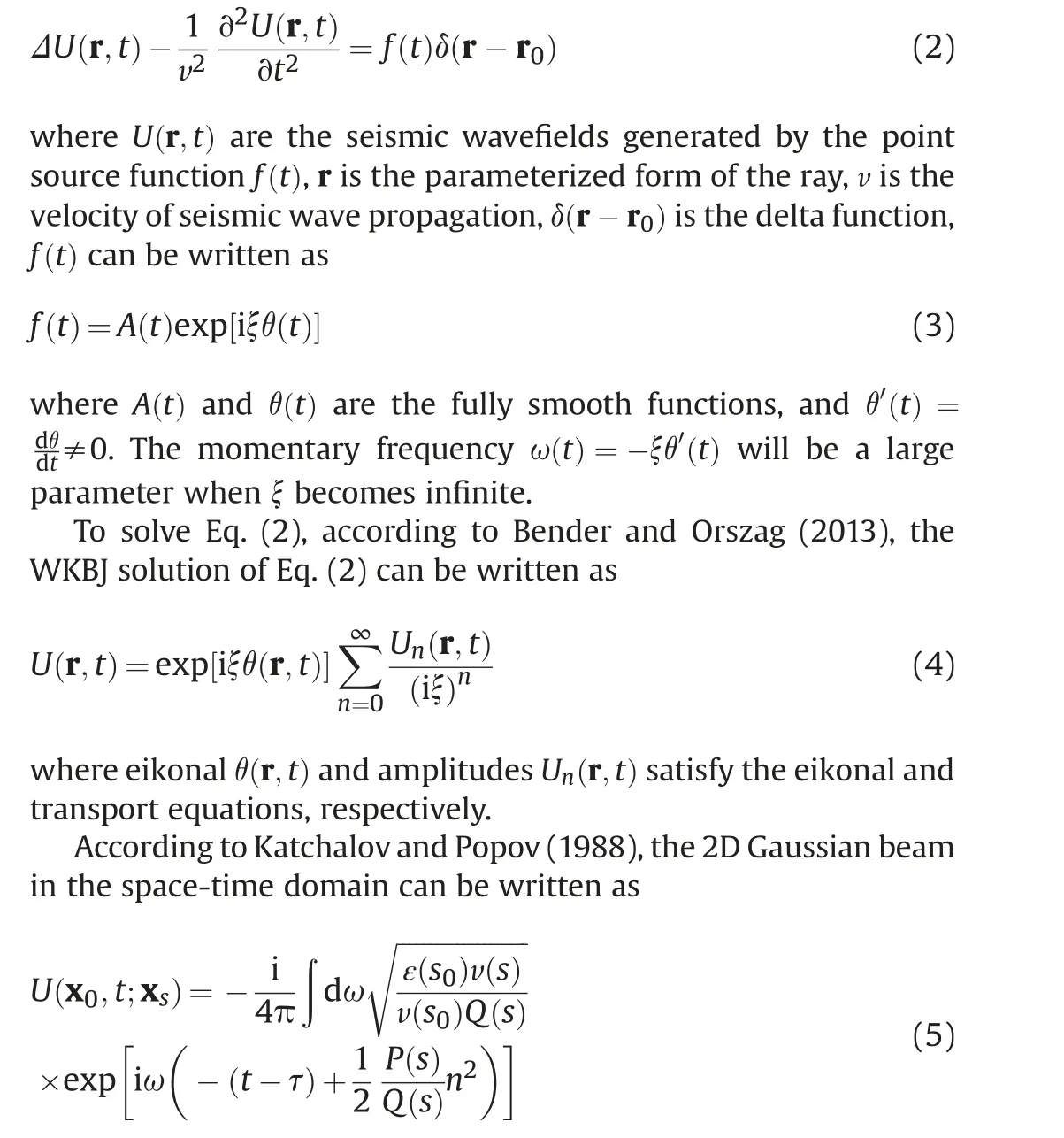
According to ˇCervený et al. (1982), in the 2D ray centered coordinate system(s'n)(Fig.1),s is the length of arc along the ray at the reference point,n represents the length in the vertical direction with s. The time of ray propagationg can be written as

where t is time,τ(s) denotes the traveltime, and v0(s) denotes the initial velocity of seismic wave propagation.
In 2D acoustic media, we consider the space-time-domain ray method for the constant-density acoustic wave equation with the piont source function f(t) as
where x0=(x0'z0) denotes the spatial rectangular coordinate at the imaging points, xs=(xs'0) denotes the spatial position coordinate at the shot points,ω is the angular frequency,ε is the initial beam parameter.The scalar fuctions P(s)and Q(s)are complex,and they can be written as
where(p(1)(s)'q(1)(s)) and (p(2)(s)'q(2)(s)) are two solutions of the dynamic ray tracing equations with spherical and plane-wave initial conditions.Hill(1990)gave the expression of ε and the initial value of q(s0) and p(s0) as
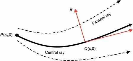
Fig.1. The 2D ray centered coordinates in the vicinity of a ray.

We establish the relationship between(s;0)and(s0;0)by Eq.(8)and Eq. (9). If we know one, we can get another.
2.2. Construction of wavefields
The forward wavefields W(F)(x0't;xs) could be composed of a series of Gaussian beams from different angles and frequencies(ˇCervený et al.,1982; Popov,1982), which could be expressed as


where pzare the vertical ray parameter at receiver points.
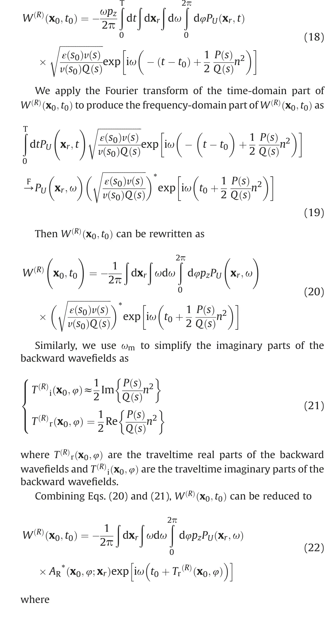
Inserting Eq. (16) and Eq. (17) into Eq. (15), the expression of W(R)(x0't0) can be written as
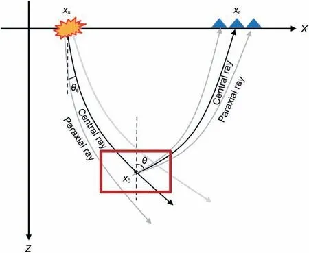
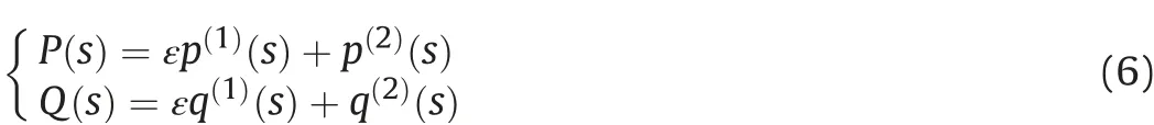
Fig. 2. Diagram of the upward ray tracing strategy.
2.3. Space-time-domain GBM
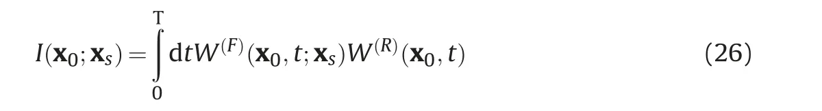
Thus,we use the cross-correlation imaging condition to get the imaging results as
To reduce the coherent noise,we get the final imaging results by stacking the multiple-shot imaging profiles.I(x0)can be expressed as

2.4. Ray parameter optimization
For the take-off angle increment of the up-going and downgoing rays, we use the angle spacing of the central rays in the frequency-domain GBM(Hill,1990) as
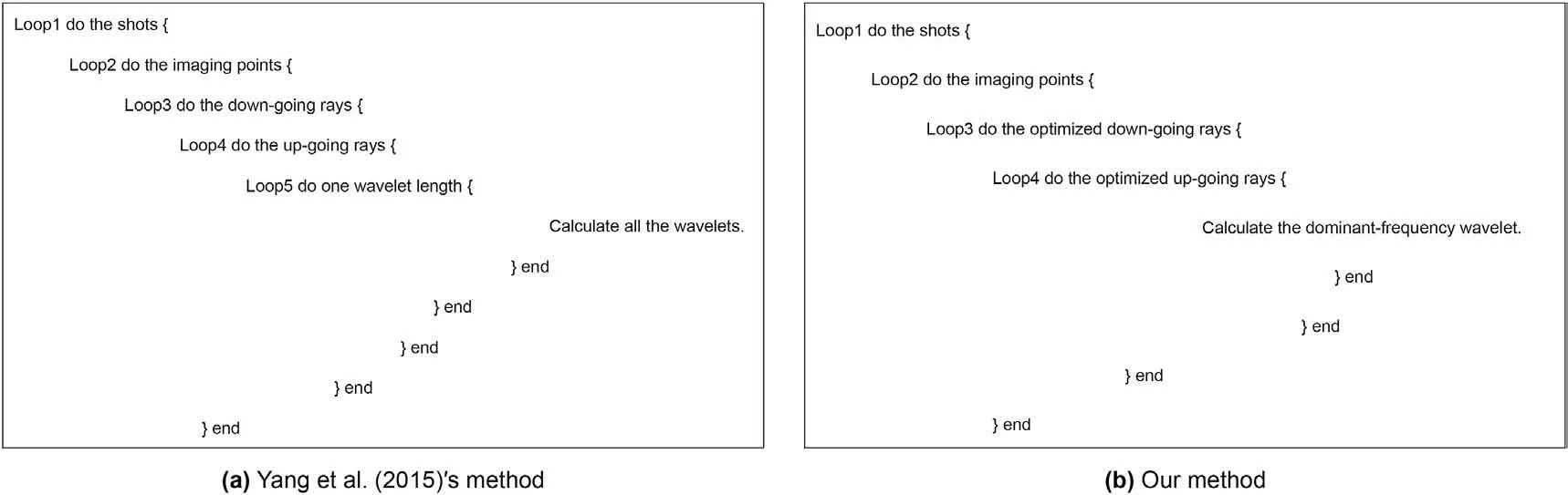
Fig. 3. The flowchart.
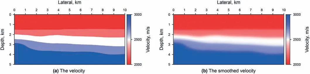
Fig. 4. The simple layers model.
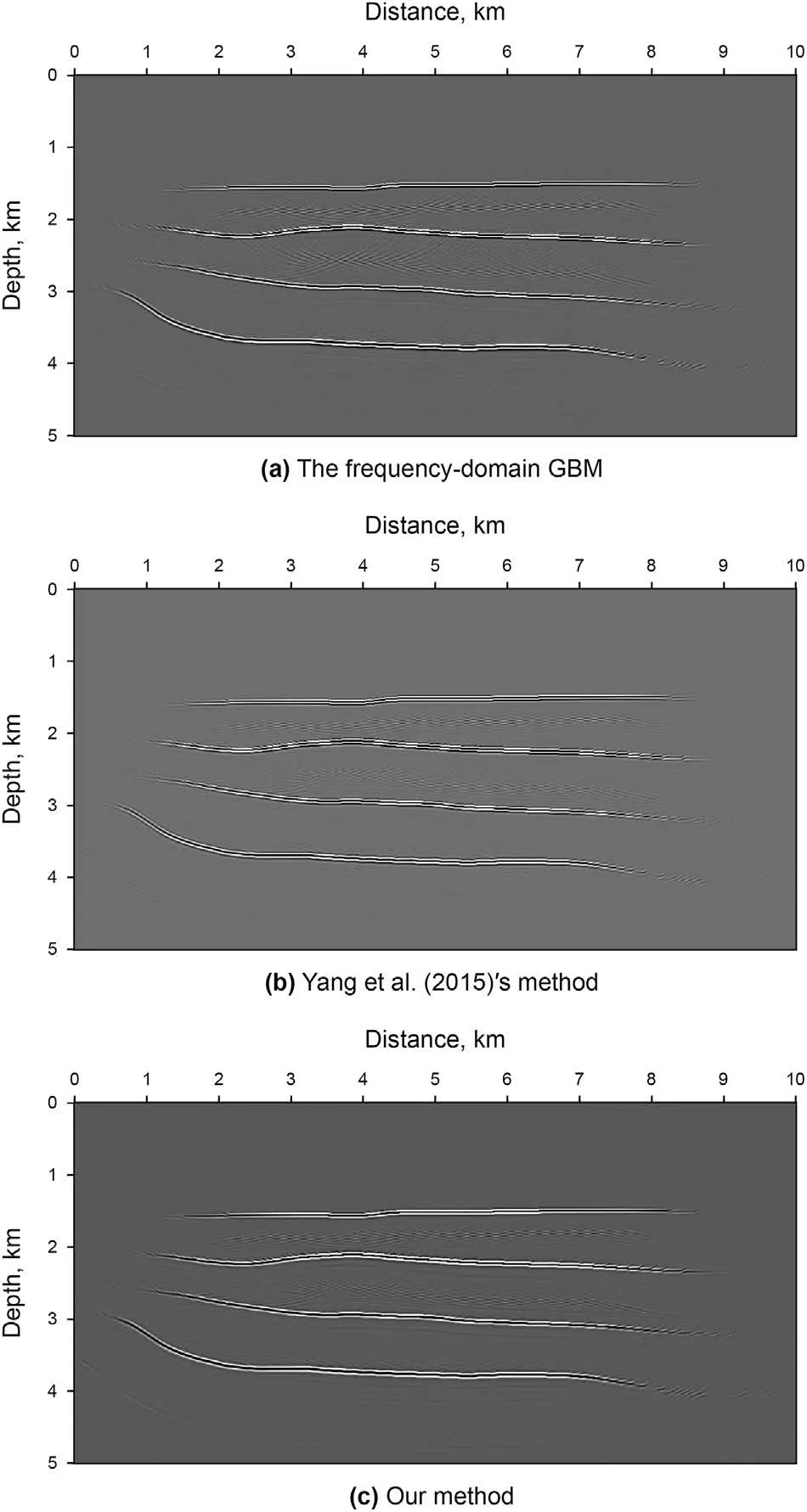
Fig. 5. Multiple-shot migration results for the simple layers model.
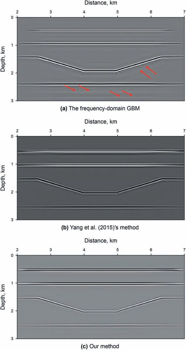
Fig. 7. Multiple-shot migration results for the graben model.
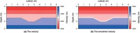
Fig. 6. The graben model.
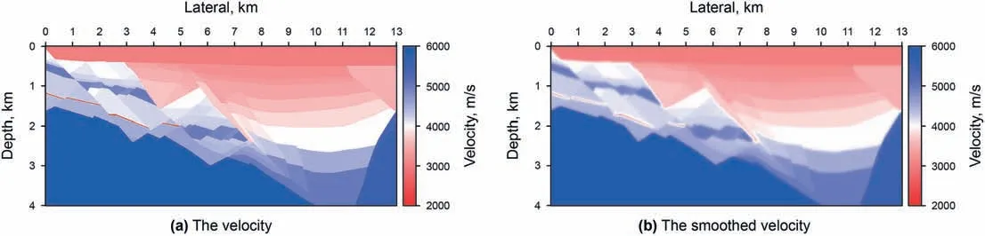
Fig. 8. The buried hill model.
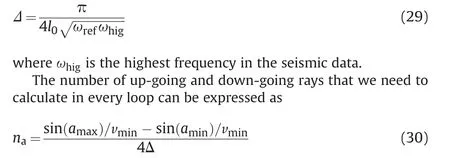
where amaxis the maximum offset angle, aminis the minimum offset angle, vminis the minimum velocity.
With the premise of ensuring imaging accuracy,the calculation time of the amplitude and traveltime of the up-going and downgoing rays in the loop algorithm is reduced, further improve the computational efficiency of our method.
Finally, we give the implementation process of the proposed method (Fig. 3b). Compared with Yang et al. (2015)'s method(Fig.3a),we see that our method realizes one cycle in the algorithm than Yang et al. (2015)'s method and we choose an optimized parameter of the take-off angle increment for the up-going and down-going rays, which can help us obtain a faster space-timedomain GBM approach.
3. Numerical examples
In the first example,we use the simple layers model as shown in Fig. 4 to test the correctness of our method. The grid size of this model is 1001 × 501 with the spacing size of 10 m. There are 26 shots,and the shot spacing is 200 m.There are 501 traces per shot,and the trace spacing is 10 m.The recording time length is 5 s,and the sampling interval is 0.5 ms.Fig.5 are the results which we use the frequency-domain GBM, Yang et al. (2015)'s method and our method. In Fig. 5b and c, we see that our new method produces good imaging results with comparable accuracy to the Yang et al.(2015)'s method, indicating that our method is correct for the simple model. Besides, compared with the running time of two space-time-domain GBM methods, our new method can increase the computational efficiency by 211.4 times for the simple layers model (Fig. 4).
Then,we use the graben model(Fig.6)to test the adaptability of our method for the simple models. It has the grid size with 1801 × 301. The horizontal spacing is 5 m and the vertical grid spacing is 10 m. The shots number is 201 and each shot has 301 traces.The shot and trace spacing are 25 m and 10 m,respectively.The time sampling interval is 1 ms and the number of time sample is 2500. Fig. 7a and b are the migration results of the frequencydomain GBM and the space-time-domain GBM method proposed by Yang et al. (2015). The frequency-domain GBM produces some imaging artifacts(red arrows)in Fig.7a.In Fig.7b and c,we see that they can clearly image all reflectors with good accuracy due to the upward ray tracing strategy for time reversal wavefields. At the same time,the comparisons of the running time of two space-timedomain GBM methods show that our new method can improve the computational efficiency by 136.0 times for the graben model(Fig. 6).
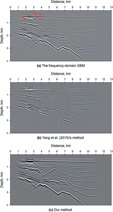
Fig. 9. Multiple-shot migration results for the buried hill model.
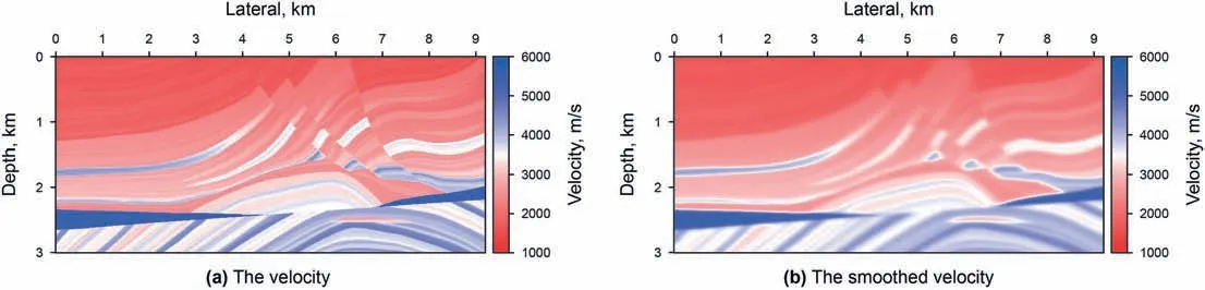
Fig.10. The Marmousi model.

Fig.11. Multiple-shot migration results for the Marmousi model.
In the third example,we use the buried hill model(Fig.8)to test the adaptability of our method for imaging some complex structures.The grid size of this model is 1301×401 and the grid spacing is 10 m.There are 30 shots,and the shot spacing is 300 m.There are 401 traces per shot, and the trace spacing is 10 m. The time sampling interval is 0.5 ms and the number of time sample is 6001.Fig. 9 shows the results of the frequency-domain GBM, Yang et al.(2015)'s method and our method. We can see that frequencydomain GBM produces some shallow wide-angle reflections (red arrows) in Fig. 9a. Compared with Fig. 9a and b, the space-timedomain GBM method produces good imaging quality for the shallow layers.And our method produces the comparable results to the Yang et al.(2015)'s method(Fig.9b and c).Compared with the running time of two space-time-domain GBM methods, our method can improve the computational efficiency by 174.7 times for the buried hill model (Fig. 8).
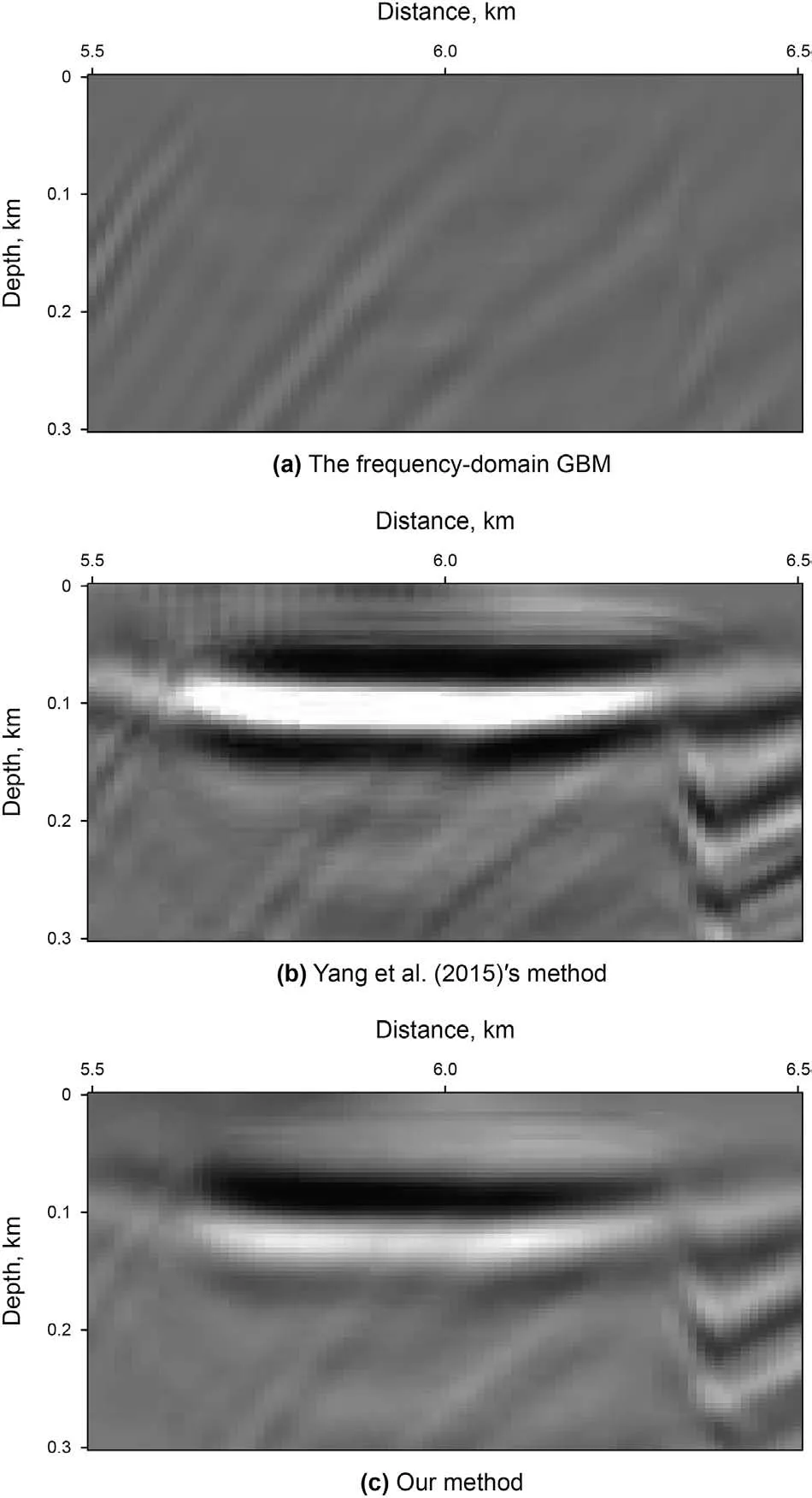
Fig.12. Magnification of migration images from Fig.11 (blue rectangle).
The final example is the 2D Marmousi model in Fig.10.It has the grid size with 737×750.The horizontal grid spacing is 12.5 m and the vertical grid spacing is 4.0 m. Here, the CDP spacing is 25 m.There are 240 shots and each shot has 96 traces.The time sampling interval (4 ms) is much larger than the first three models and the total time record is 2.5 s. Fig.11 are the results which we use the frequency-domain GBM, Yang et al. (2015)'s method and our method. We see that two space-time-domain GBM methods produce better imaging quality for the shallow layers than the frequency-domain GBM in Fig.11(blue and red rectangles).Fig.12 and Fig.13 are the magnification of migration images from the blue and red rectangles in Fig.11, respectively. We see that two spacetime-domain GBM methods approximately have the same imaging accuracy as shown Fig. 11. However, our method slightly decreases the imaging energy at the top of the deep anticline because our approximations may result in less Gaussian beam stacking at some complex areas. Compared with the running time of two space-time-domain GBM methods, our method can improve the computational efficiency by 39.9 times for the Marmousi model(Fig.10).
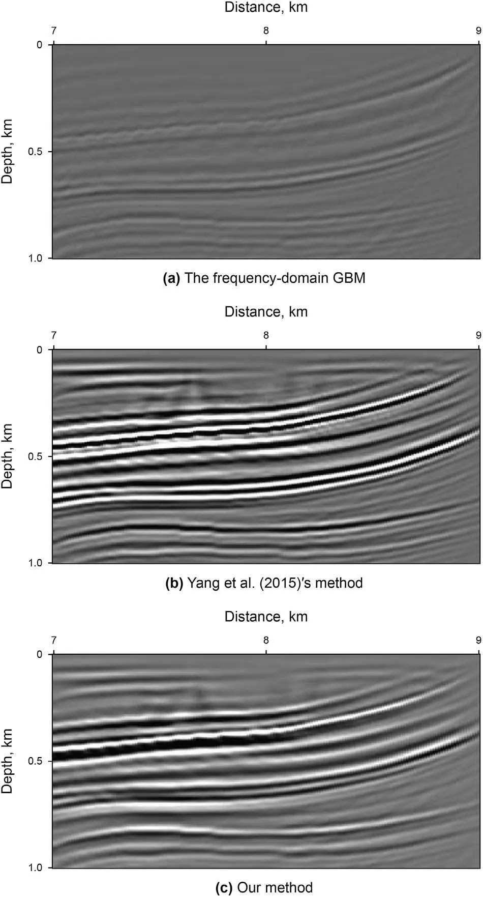
Fig.13. Magnification of migration images from Fig.11 (red rectangle).
4. Discussion
4.1. The sensitivity of the model parameters
Fitstly,we're going to focus on what parameters affect the final computational efficiency of our method.
We define the following formula as
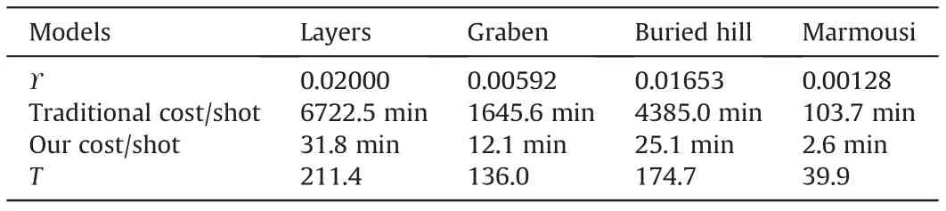
Table 1 The parameters of two space-time GBM methods.
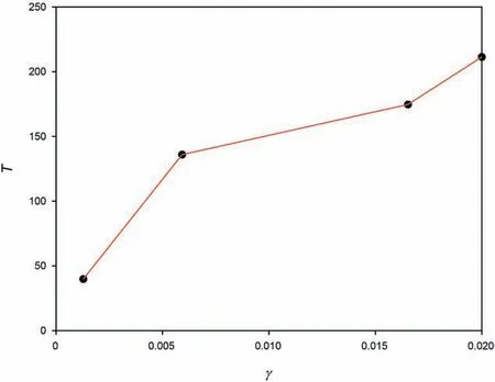
Fig.14. The function of T as γ varies.
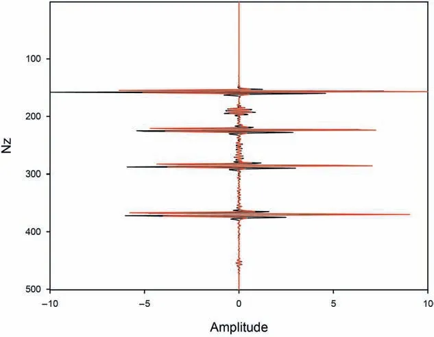
Fig. 15. The results of wavelet comparisons for Fig. 5 in Yang et al. (2015)'s method(black) and our method (red).

Fig.16. The results of wavelet comparisons for Fig.12 in Yang et al. (2015)'s method(black) and our method (red).
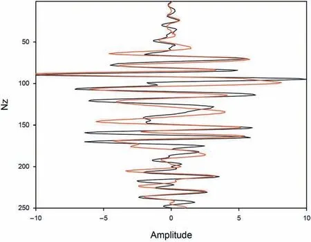
Fig.17. The results of wavelet comparisons for Fig.13 in Yang et al. (2015)'s method(black) and our method (red).

where Ntdenotes the wavelet length, which is negatively associated with the time sampling interval in the traditional space-timedomain GBM.
And the running time of two space-time-domain GBM methods of a single shot can be seen in Table 1. We define the ratio of the running time of the traditional space-time-domain GBM to the running time of our method as

where T1is the running time of the traditional space-time-domain GBM for a single shot, T2is the running time of our method for a single shot.
In Fig.14,the profile suggests that the improved computational efficiency of our method T is positively correlated with γ. It is just the result that we do some approximations and optimizations.
4.2. The influence of the comlexity of the models
Secondly, we will discuss the cost difference caused by the different model complexity.In our new algorithm,the running time(Ttotal)can be mainly divided into two parts(Trayand Tmigration).The first part(Tray)is the cost for the ray tracing,which is the same cost between our new method and Yang et al. (2015)'s method. The second part (Tmigration) is the cost of the migration process. In our new method, we first decrease the loop layer from 5 of Yang et al.(2015) to 4; in addition, we also highly improve the computational efficiency by decreasing the up-going and down-going rays density in loop 3 and loop 4 in Fig.3b.For different models with the same paremeters, Trayis basically same with two space-timedomain GBM methods, which mainly depends on the complexity of the models. As the model gets more complex, Traybecomes bigger. At the same time, our approximations and optimizations mainly reduce Tmigration. Thus, it will slightly reduce the improved computational efficiency of our method with more complex models.
4.3. The quantitative analysis of our method
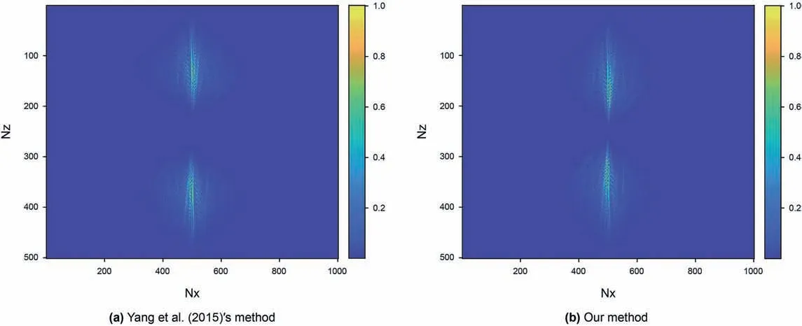
Fig.18. Comparisons of wavenumber spectrum for Fig. 5 (all panels are normalized according to their maximum values).

Fig.19. Comparisons of wavenumber spectrum for Fig.12 (all panels are normalized according to their maximum values).

Fig. 20. Comparisons of wavenumber spectrum for Fig.13 (all panels are normalized according to their maximum values).
Finally, we give the quantitative analysis of our method using the simple layers and Marmousi models as the examples. Fig.15,Fig.16 and Fig.17 are the results of wavelet comparisons for Fig.5,Fig. 12 and Fig. 13 in two space-time-domain GBM methods,respectively. We can find that our method has slight influence on the wavelet phase in some locations, which approximately influences 1%-3% for lithology imaging. But it is worth that we significantly improve the computational efficiency up to one or even two orders of magnitude. Fig.18, Fig.19 and Fig. 20 are the comparisons of wavenumber spectrum for Fig.5,Fig.12 and Fig.13 in two space-time-domain GBM methods, respectively. In general,two methods have a nearly same range of wavenumbers because our method only simplifies the computation of the forward and backward wavefields associated with the imaginary traveltime,the real traveltime still contains the information with all frequencies.
5. Conclusions
We propose a fast and accurate space-time-domain acoustic GBM method with some approximations and optimizations. Four numerical examples show that the proposed method can significantly reduce the computational cost of the traditional space-timedomain GBM.And different models can improve the computational efficiency differently, it mainly depends on the selections of the parameters of different models. Compared with the frequencydomain GBM, our method produces good imaging quality for the shallow layers and it has better imaging accuracy. In addition, our new method produces good imaging results with comparable accuracy and resolution with the traditional space-time-domain GBM.
It is difficult to apply the traditional space-time-domain GBM to large-scale field data processing due to the larger computational cost.Experiments show that compared with the traditional spacetime-domain GBM, our new method can improve the computational efficiency by 39.9-211.4 times in different models. It solves the key problem of the development of the space-time-domain GBM and has a good potential. Thus, our method will be a new fast and flexible tool for seismic imaging in geologically complex areas.
Acknowledgements
This study is jointly supported by the National Key Research and Development Program of China (2019YFC0605503), the National Natural Science Foundation of China (41821002, 41922028,41874149), the Strategic Priority Research Program of the Chinese Academy of Sciences (XDA14010303), the Major Scientific and Technological Projects of CNPC (ZD2019-183-003). We thank the editors of Petroleum Science and the reviewers,whose constructive comments improve the paper.
杂志排行
Petroleum Science的其它文章
- Predicting gas-bearing distribution using DNN based on multicomponent seismic data: Quality evaluation using structural and fracture factors
- Reflection-based traveltime and waveform inversion with secondorder optimization
- Determination of dynamic capillary effect on two-phase flow in porous media: A perspective from various methods
- Settling behavior of spherical particles in eccentric annulus filled with viscous inelastic fluid
- Laboratory investigation on hydraulic fracture propagation in sandstone-mudstone-shale layers
- Damage of reservoir rock induced by CO2 injection