Huber inversion-based reverse-time migration with de-primary imaging condition and curvelet-domain sparse constraint

Bo Wu , Gang Yao ,*, Jing-Jie Cao , Di Wu , Xiang Li , Neng-Chao Liu

a State Key Laboratory of Petroleum Resources and Prospecting, China University of Petroleum (Beijing), Beijing,102249, China

b Unconventional Petroleum Research Institute, China University of Petroleum (Beijing), Beijing,102249, China

c Key Laboratory of Intelligent Detection and Equipment for Underground Space of Beijing-Tianjin-Hebei Urban Agglomeration, Ministry of Natural Resources, Hebei GEO University, 050031, China

d Hebei Key Laboratory of Strategic Critical Mineral Resources, Hebei GEO University, Shijiazhuang, Hebei, 050031, China

e College of Geophysics, China University of Petroleum (Beijing), Beijing,102249, China

Keywords:Least-squares reverse-time migration Huber-norm Sparse constraint Curvelet transform Iterative soft thresholding

ABSTRACT Least-squares reverse-time migration (LSRTM) formulates reverse-time migration (RTM) in the leastsquares inversion framework to obtain the optimal reflectivity image. It can generate images with more accurate amplitudes,higher resolution,and fewer artifacts than RTM.However,three problems still exist: (1) inversion can be dominated by strong events in the residual; (2) low-wavenumber artifacts in the gradient affect convergence speed and imaging results;(3)high-wavenumber noise is also amplified as iteration increases. To solve these three problems, we have improved LSRTM: firstly, we use Hubernorm as the objective function to emphasize the weak reflectors during the inversion; secondly, we adapt the de-primary imaging condition to remove the low-wavenumber artifacts above strong reflectors as well as the false high-wavenumber reflectors in the gradient; thirdly, we apply the L1-norm sparse constraint in the curvelet-domain as the regularization term to suppress the high-wavenumber migration noise.As the new inversion objective function contains the non-smooth L1-norm,we use a modified iterative soft thresholding (IST) method to update along the Polak-Ribi‵ere conjugate-gradient direction by using a preconditioned non-linear conjugate-gradient (PNCG) method. The numerical examples,especially the Sigsbee2A model, demonstrate that the Huber inversion-based RTM can generate highquality images by mitigating migration artifacts and improving the contribution of weak reflection events.

1. Introduction

Seismic migration is a key technology in seismic data processing. It can image the subsurface structures by restoring the reflection events recorded on the surface to the true underground location. To obtain high-quality subsurface images, migration imaging technologies have evolved from ray-based Kirchhoff migration (Keho and Beydoun,1988;Schneider,1978)to Gaussian beam migration(Hill,1990,2001;Bai et al.,2019;Zhang et al.,2019),and from one-way wave-equation based migration (Claerbout, 1971;Claerbout and Doherty, 1972; Gazdag, 1978) to reverse-time migration (RTM), which is based on two-way wave equation(Baysal et al., 1983; McMechan, 1983; Whitmore, 1983; Xu et al.,2011; Shi et al., 2019; Zhao et al., 2021). At present, RTM is one of the most popular migration methods for imaging models with complex structures. The reason is that RTM employs the two-way wave equation; therefore, it can handle steeply dipping structures, adapt to strong velocity variation, accurately migrate all frequencies and deal with complex waves, such as prism waves(Zhang et al., 2011).

However,instead of inverse operators,RTM still applies adjoint operators that only preserve the kinematics of the seismic image correctly, resulting in inaccurate amplitudes and degraded resolution (Etgen et al., 2009). Especially, in cases of significant aliasing,truncation, noise, and incomplete seismic data, the adjoint of the modeling operators approximate the inverse operators roughly(Claerbout and Karrenbach, 1992). In such cases, even with an accurate migration velocity model,the image quality of RTM is still affected.

To further improve the quality, RTM is formulated in the leastsquares inversion framework to produce the optimal reflectivity image, which is referred to as least-squares reverse-time migration(LSRTM)(Dai and Schuster,2013;Liu et al.,2013;Zhang et al.,2015;Yao and Jakubowicz,2016;Yang et al.,2019b;Hu et al.,2021;Wang et al., 2021). LSRTM can generate images with more balanced amplitudes, higher resolution, and fewer artifacts caused by missing data, truncation, noise, and operator mismatch than conventional RTM,thanks to the inverse operator applied by LSRTM(Yao and Wu,2015; Wang and Wang, 2017; Yang et al., 2019a; Guo and Wang,2020; Liu et al., 2020). LSRTM could also include anisotropy (e.g.,Qu et al., 2017), attenuation (e.g., Qu and Li, 2019), elasticity (e.g.,Fang et al.,2019;Gu et al.,2019),and multiples(e.g.,Qu et al.,2021;Zhang et al.,2021)for honoring the physics more accurate.

However,conventional LSRTM utilizes L2-norm as the objective function. Consequently, the inversion is dominated by strong seismic events or other outliers in recorded data. For instance, the events originating from the boundary of salt bodies are much stronger than the events from the interfaces of sedimentary strata under the salt bodies. These strong events dominate the whole inversion process of LSRTM, resulting in an inadequate update to the region under the salt domes.

The second weakness of conventional LSRTM is that it still uses the zero-lag cross-correlation imaging condition, which generates the low-wavenumber migration artifacts, especially above strong reflectors, due to the two-way wave equations employed. In addition, the zero-lag cross-correlation imaging condition also generates false high-wavenumber reflectors in geologically complex areas(Fei et al.,2010).Although conventional LSRTM can suppress the low-wavenumber migration artifacts to some degree through the fitting process, this will affect the convergence speed of inversion in the early iterations.

The wavefield decomposition method is a popular choice to mitigate the low-wavenumber migration artifacts. Liu et al. (2011)proposed an efficient wavefield decomposition method to suppress low-wavenumber migration artifacts in the RTM images. Fei et al. (2015) proposed the de-primary imaging condition to further improve the effectiveness of imaging. Except for suppressing low-wavenumber migration artifacts, this imaging condition can also eliminate false high-wavenumber reflectors. Kim et al.(2019) used the de-primary imaging condition in LSRTM and utilized a preconditioned linear conjugate-gradient method(PLCG)for inversion.However,the migration operator is no longer the adjoint of the modeling operator as the de-primary imaging condition changes the gradient of LSRTM. This method slows down the convergence of inversion. To mitigate this problem, they used the de-primary imaging condition only at early iterations, and then switched to the zero-lag cross-correlation imaging. However, the later iterations with the zero-lag cross-correlation imaging condition still introduce low-wavenumber artifacts again.

Thirdly, the inversion process of conventional LSRTM also produces high-wavenumber noise to overfit the record because of the ill-conditioning nature of geophysics problems as well as the modeling engine that only simulates the record partially (Trad,2020). To solve this problem, L1-norm sparse constraints are incorporated into LSRTM to penalize the high-wavenumber migration noise and reduce the sidelobes around the reflectors(Lin and Lian,2015;Wu et al.,2016;Dutta,2017;Li et al.,2017).This method suppresses the artifacts and also the weak reflectors. Li et al. (2020) further implemented the L1-norm sparse constraint in the wavelet domain. It can perform multi-scale and angle analysis, so it can protect weak signals better while removing noise.

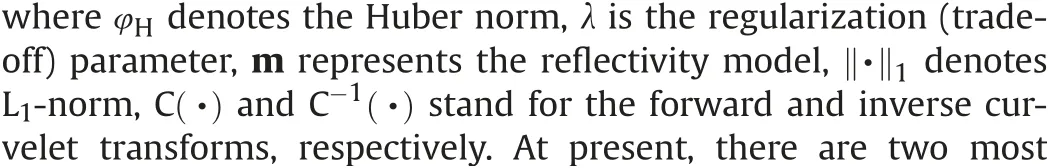
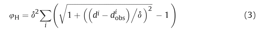
In this paper, we propose a new strategy to achieve LSRTM for solving these problems illustrated above. Firstly, we employ a Huber norm (Huber,1964) as the objective function of the inversion. Thus, the inversion acts as L1-norm inversion for large residuals but as L2-norm inversion for small residuals.Consequently,it is strongly convex when close to the minimum and less steep for large residuals.Thus,this can mitigate the problem:large residuals dominate the inversion of LSRTM.Since the inversion is not based on L2-norm only, we call it Huber inversion-based RTM instead of LSRTM.Secondly,the de-primary imaging condition is employed to formulate the gradient instead of the zero-lag cross-correlation imaging condition, which causes both low-wavenumber artifacts and high-wavenumber false reflectors.Finally,we use the L1-norm sparse constraint in the curvelet-domain as the regularization term to remove high-wavenumber noise.The reason is that the curvelet transform can sparsely represent images at multiple scales and angles,and has a stronger ability to express edge information than other transforms, such as wavelet transform (Cand‵es and Guo,2002). As the proposed Huber inversion-based RTM contains a non-smooth L1-norm, we utilize an improved iterative soft thresholding (IST), which is updated along the Polak-Ribi‵ere conjugate-gradient direction by using a preconditioned non-linear conjugate-gradient (PNCG) method. The numerical examples,especially the Sigsbee2A model, demonstrate that our proposed method can improve the image quality and show more structural details in poorly illuminated areas.

In the following chapters, firstly, we introduce the theory of Huber inversion-based RTM with the curvelet-domain constraint.Secondly, numerical examples are presented to prove the effectiveness of the proposed method.Before the conclusion,we discuss the convergence of all these RTM methods,the effectiveness of the curvelet-domain sparse constraint for noise suppression with Huber inversion-based RTM,and the influence of velocity accuracy on inversion-based RTM methods.

2. Method

2.1. Huber inversion-based reverse-time migration with curveletdomain constraint

Least-square reverse-time migration(LSRTM)generally uses the L2-norm objective function.

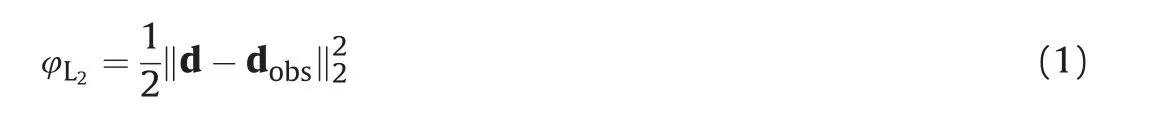
where d denotes the predicted data and dobsrepresents the observed data.Note that a boldface letter in an equation represents the vector form of a variable,whereas a normal letter is for its scalar form in the whole paper. The L2-norm objective function is particularly efficient for reflection events that have similar amplitudes from sedimentary rocks. However, if models include large contrast in geological bodies, e.g. salt bodies, then an objective function which emphasizes more on weak events is expected. Besides, a constraint should be incorporated into the migration inversion system to suppress high-wavenumber noise generated by the inversion process. By considering the two points, we combine the Huber norm and the curvelet-domain constraint as the objective function

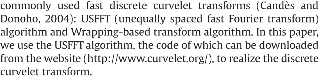
In this paper, we choose a pseudo-Huber loss function(Charbonnier et al.,1997)to replace the L2-norm objective function

where diand diobsrepresents the ith element of d and dobs,respectively,and δ is the threshold of Huber-norm.An advantage of the pseudo-Huber norm over the pice-wise Huber norm is that its gradient is continuous for all values, which is convenient for implementing gradient-based inversion methods. We choose half the maximum value of the residual,i.e.data misfit di-diobs,as δ in each iteration. Therefore, when the residual is large, the Huber norm acts like L1-norm; otherwise, it acts like L2-norm. Since the residual shrinks as inversion progresses,δ decreases during inversion. Reducing δ as inversion progresses is an effective strategy in optimization called“cooling”.In the early iterations, the value of δ is relatively large, therefore, strong events converge quickly. As inversion progresses,reducing δ increases the contribution of weak signals in the objective function and avoids strong events continuing to dominate the updating direction of the model. Note that δ in the pseudo-Huber norm is slightly larger than the transition point between the two norms.This is illustrated by Fig.1.

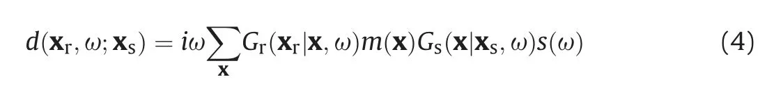
The mapping relationship between predicted data and reflectivity is essential for minimizing the objective function. Generally,there are two simulation methods for predicted data:one is based on Born approximation, and the other is based on Kirchhoff approximation(Jaramillo and Bleistein,1999;Bleistein et al.,2005).In this paper, we used the Kirchhoff approximation:

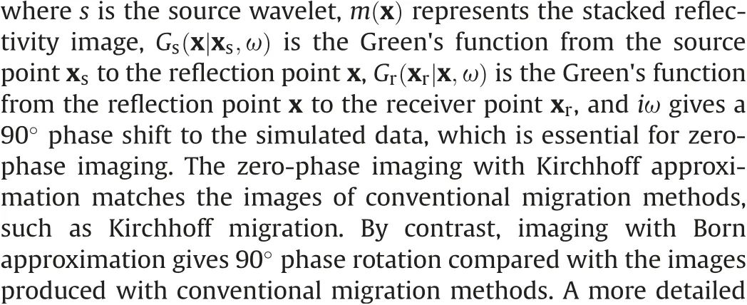
Eqs. (2)-(4) constitute the inversion system used in this paper.To minimize the function in Eq. (2), we employ the iterative soft thresholding (IST) method, which is an effective approach to minimizing the mixed norm problems. IST is a special type of the proximal method, which solves a general optimization problem

2.2. Gradient approximated by de-primary imaging condition

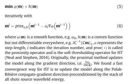
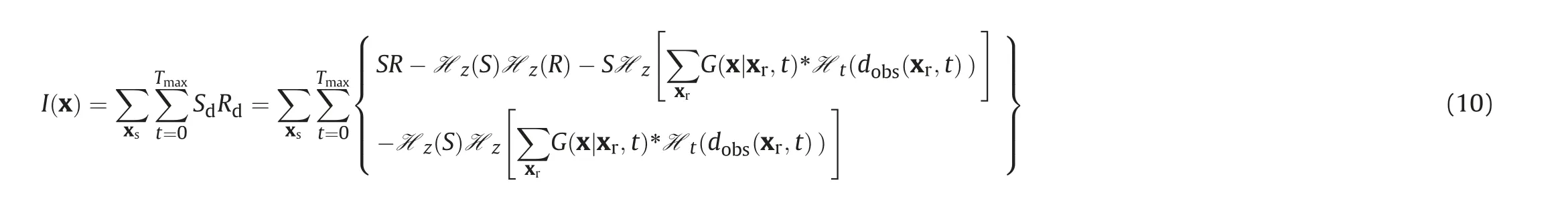
Substituting Eq. (4) into Eq. (3) can yield the gradient of the objective function

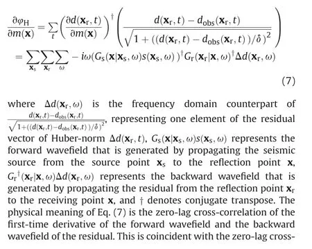
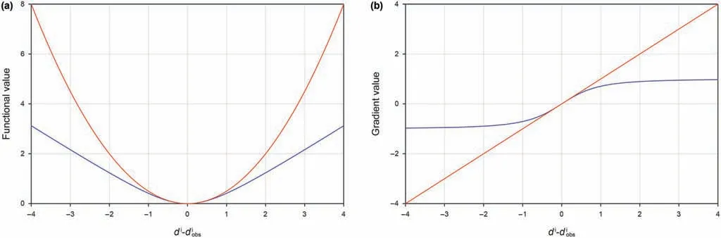
Fig.1. A sketch of the pseudo-Huber loss function (blue, δ = 1) and the L2-norm loss function 12 d-dobs 22 (red). (a) The functional value and (b) their gradients.

correction imaging condition widely used in reverse-time migration (RTM). For a common shot gather, it can be expressed as

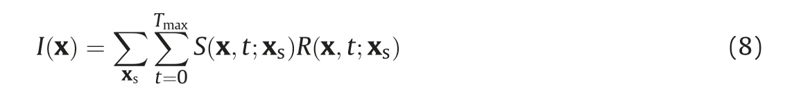
where I（x） represents the RTM image, S（x't;xs） indicates the source wavefield (or the forward wavefield), and R（x't;xs） stands for the receiver wavefield (or the backward wavefield). Eq. (8) can be expressed by wavefield decomposition as follows (Liu et al.,2011)

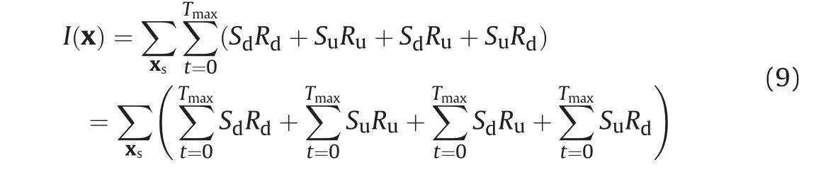
where the subscripts u and d indicate the up-going and downgoing wavefields. SdRdproduces the primary reflectors, SuRuusually generates false reflectors in RTM, SdRuand SuRdproduce lowwavenumber migration artifacts. The process of producing the false reflectors is shown in Fig. 2. Therefore, the de-primary imaging condition only retains the first term of Eq.(9).This term can be expressed by using Hilbert Transform (Fei et al., 2015)

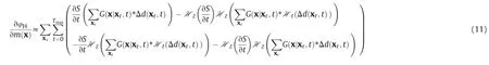
In the same way, in order to suppress the low-wavenumber artifacts and high-wavenumber false reflectors from the gradient of Huber inversion-based RTM, we apply de-primary imaging condition by decomposing the first-order time derivative of the forward wavefield and the backward wavefield into the up-going and down-going wavefields through the Hilbert Transform, and then only keeping the first term. Therefore, the gradient of Huber inversion-based RTM with the de-primary imaging condition can be written approximately as

It can be seen from Eq.(7)that the gradient with the de-primary imaging condition in Eq. (11) is not the exact gradient of the objective function,therefore,PLCG methods are not the best choice for inversion. Its convergence will be affected. This situation happens not only in the Huber inversion-based RTM but also in the traditional LSRTM with the de-primary imaging condition.To solve this problem, the PNCG method is a better choice to ensure the convergence of the inversion.

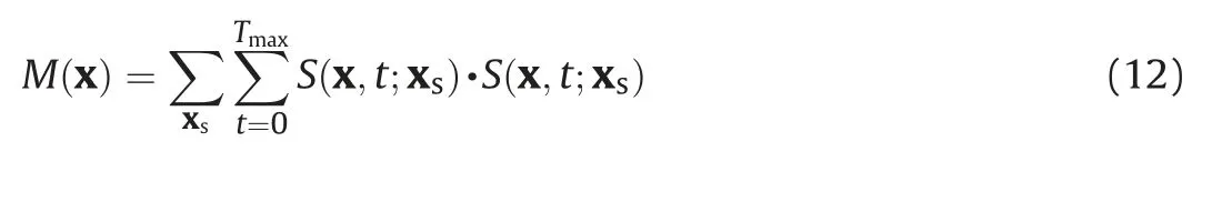
By combining all the aspects presented above,we minimize the function in Eq. (2) by using IST with the Polak-Ribi‵ere conjugategradient direction preconditioned by the stack of all shots source wavefield energy. The detailed algorithm is listed in Algorithm 1.Generally, the optimal value of λ is refined by trial and error. The preconditioner M is defined as

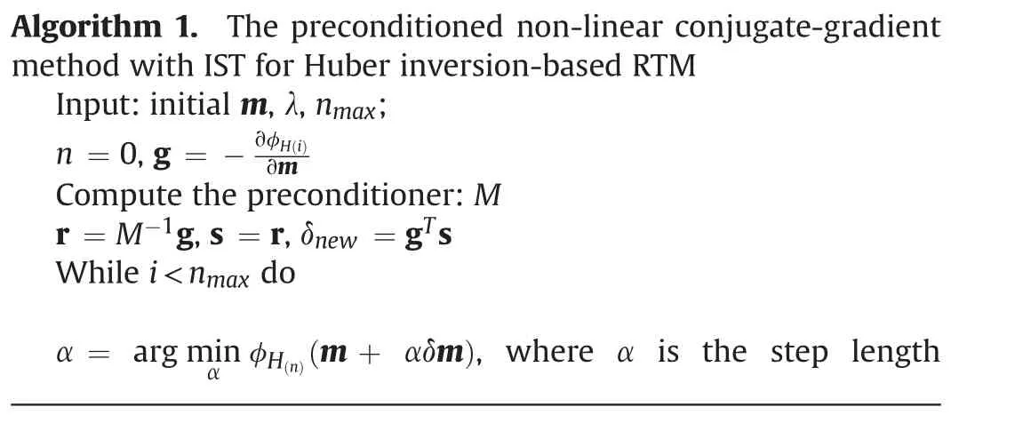
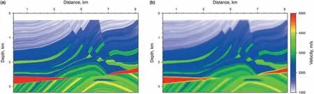
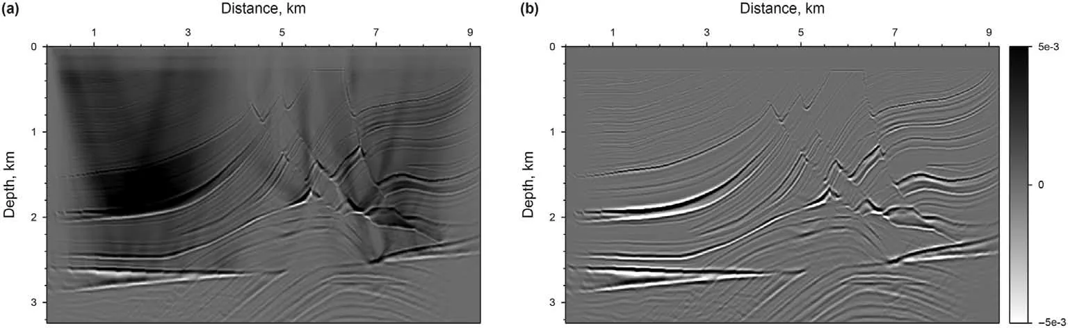
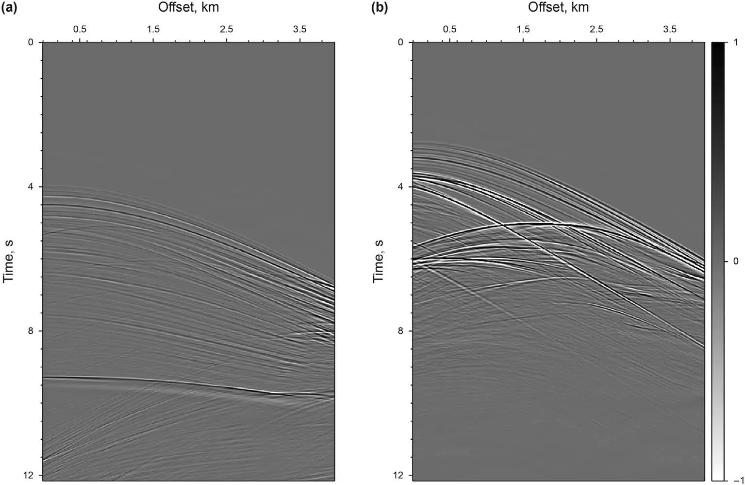
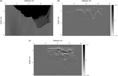
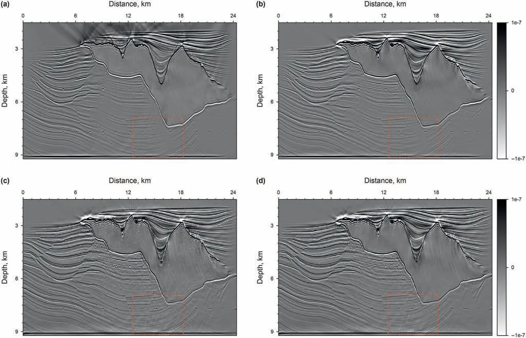
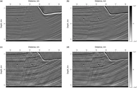
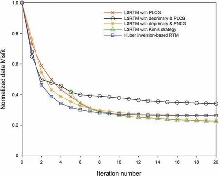
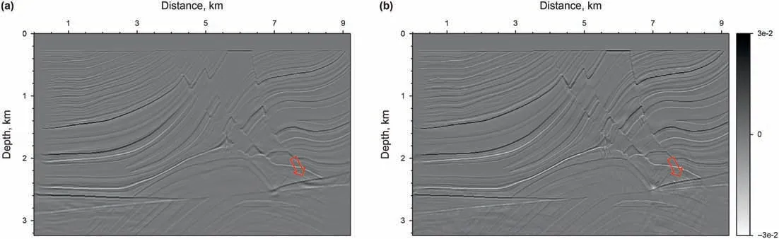
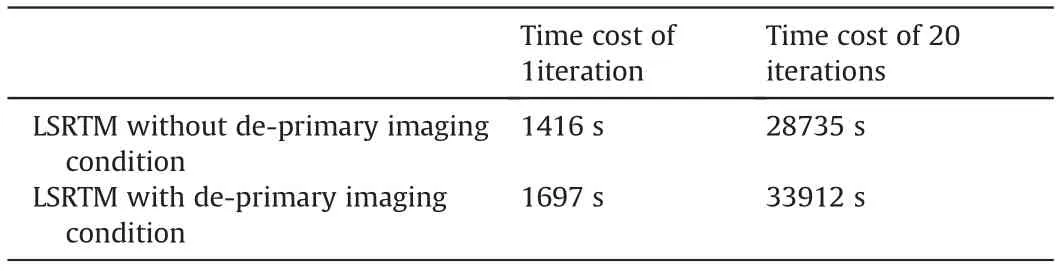
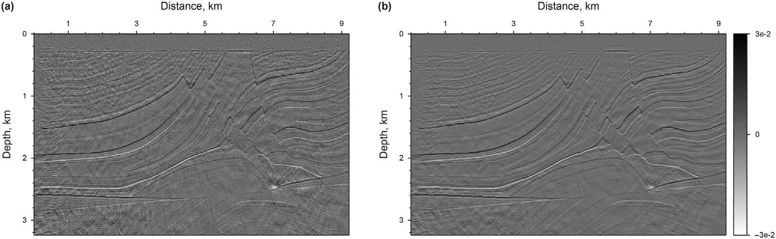
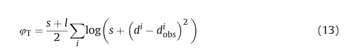
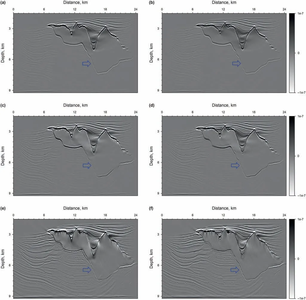
Algorithm 1. The preconditioned non-linear conjugate-gradient method with IST for Huber inversion-based RTM Input:initial m,λ, nmax;n = 0, g = -∂φH（i）∂m Compute the preconditioner: M r = M-1g, s = r,δnew = gTs While i

computed by line search and δm is a small perturbation along s.︿m = C（m +αδm）m = C-1（Tλ（︿m））, where Tλ（︿mi） = sgn（︿mi）max（0'■︿mi■-λ）g = -∂φH（i）∂m δold =δnew,δmid = gTr, r = M-1g,δnew = gTr β = max（（δnew -δmid）/δold'0）, s = r+βs i = i+ 1 end

Fig. 2. Schematic illustration of the de-primary imaging condition in a three-layer model. The blue dot represents the false image produced by the up-going wavefields,while the red dot denotes the true image created by the down-going wavefields.Both of them have the same travel time.

3. Numerical examples

3.1. Marmousi2 model

In the first example,the Marmousi2 model is used to demonstrate the effectiveness of the Huber inversion-based RTM.The seismic data set is generated from the Marmousi2 model with fine stratigraphy(Fig.3a)by solving the two-way acoustic wave equation.The data set includes 176 shots with a shot spacing of 50 m. A split-spread geometry is applied. The receiver spacing is 25 m. The minimum and maximum offsets are 0 m and 2600 m, respectively. The source wavelet is a 30 Hz Ricker wavelet.The total recording duration is 3.2 s with a sampling interval of 0.4 ms. The sources and receivers are positioned at 20 m below the surface. Two typical shot gathers are shown in Fig.4,in which the direct arrivals are removed.A slightly smoothed velocity model shown in Fig.3b is used for migration. In industrialapplications,themigrationvelocityisbuiltmainlywithraybased reflection tomography (Murphy and Gray,1999) or reflection waveform inversion (Yao et al., 2020). Note that we deliberately smoothed the velocity model slightly to demonstrate the inversion methods’effectiveness of suppressing low-wavenumber artifacts.

Fig. 3. The Marmousi2 model: (a) the stratigraphic velocity model; (b) a smoothed version of (a). The smooth is achieved using the Seismic Unix command “smooth2” with the parameter r1 = r2 =10. The spatial sampling interval in the horizontal and vertical directions is 6.25 m and 4 m, respectively.

Fig. 4. Two shot gathers: the source is located at the distance of (a) 2.675 km and (b) 5.675 km. The direct arrivals are removed.

Fig. 5a and b shows the RTM images with the zero-lag crosscorrelation imaging condition and the de-primary imaging condition, respectively. By comparison, low-wavenumber migration artifacts prevail because of the zero-lag cross-correlation imaging condition in Fig.5a.These artifacts cover up some real reflectors.In Fig. 5b, the de-primary imaging condition mitigates the lowwavenumber migration artifacts effectively. To further improve the imaging quality,we carried out LSRTM using the result of RTM with the de-primary imaging condition (Fig. 5b) as the initial model.Figs.6a and b depict the results of LSRTM with the zero-lag cross-correlation imaging condition and the de-primary imaging condition,respectively,after 20 iterations.As can be seen,although the initial model does not contain low-wavenumber migration artifacts, the result of LSRTM with the zero-lag cross-correlation imaging condition (Fig. 6a) introduces low-wavenumber artifacts back, which are indicated by the red arrows in Fig. 6. By contrast,LSRTM with the de-primary imaging condition removes the lowwavenumber migration artifacts completely. Furthermore, the reflectors are focused better by using the de-primary imaging condition than the zero-lag cross-correlation imaging condition. The reason is that removing the low-wavenumber artifacts helps inversion to focus on updating reflectors.Fig.6c shows the imaging result of Huber inversion-based RTM with the de-primary imaging condition. As the sedimentary strata dominates the Marmousi2 model,the events in the record share similar amplitudes.Thus,the imaging result of Huber inversion-based RTM is similar to LSRTM.However, we can still see high-wavenumber artifacts, pointed by the blue arrows in Fig. 6c. The high-wavenumber artifacts are suppressed largely by incorporating the curvelet-domain sparse constraint, which is shown in Fig. 6d.

3.2. Sigsbee2A model

In the second example, the proposed method is applied to a synthetic data set from the Sigsbee2A model, which is a very challenging model for migration due to a huge salt body in the model. A seismic data set is generated by solving the two-way acoustic wave equation with the fine stratigraphic velocity model(Fig.7a).The data set includes 160 shots,which are excited with a shot spacing of 137.16 m. A one-side geometry is used with a receiver spacing of 45.72 m. The minimum and maximum offsets are 0 m and 3989 m, respectively. The source wavelet is a 12 Hz Ricker wavelet.The total recording duration is 12 s with a sampling interval of 1 ms. Two typical shot gathers are shown in Fig. 8. A smoothed version of the true velocity model shown in Fig. 7b is used for migration.

Fig. 5. RTM images: (a) the zero-lag cross-correlation imaging condition and (b) the de-primary imaging condition.

Fig.6. Migration images.(a)LSRTM with the zero-lag cross-correlation imaging condition;(b)LSRTM with the de-primary imaging condition;(c)Huber inversion-based RTM with the de-primary imaging condition;(d)Huber inversion-based RTM with the de-primary imaging condition and the curvelet-domain spare constraint.The initial model is shown in Fig. 5b. All the inversions contain 20 iterations. The red arrows indicate the low-wavenumber artifacts, whereas the blue arrows point out the high-wavenumber noise.

Fig.7. The Sigsbee2A models.(a)The stratigraphic velocity model,(b)a smoothed version of(a)using a 20-point cosine-square window for migration.The spatial sampling interval along the horizontal and vertical directions is 11.43 m and 7.62 m, respectively.

Fig. 8. Two shot gathers. The source is located at a distance of (a) 0.274 km and (b) 13.99 km. The direct arrivals are removed.

Fig. 9. RTM images. (a) Using the zero-lag cross-correlation imaging condition; (b) Laplacian filtered result of the image in (a); (c) using the de-primary imaging condition.

Fig.10. Migration images: (a) LSRTM with the zero-lag cross-correlation imaging condition at the 20th iteration; (b) LSRTM with the de-primary imaging condition at the 15th iteration;(c)Huber inversion-based RTM with the de-primary imaging condition at the 15th iteration;(d)Huber inversion-based RTM with the de-primary imaging condition and the curvelet-domain sparse constraint at the 15th iteration.

Fig. 9a shows the RTM images with the zero-lag cross-correlation imaging condition. As can be seen, strong low-wavenumber migration artifacts in Fig. 9a affect the imaging result severely: it covers up the real high-wavenumber reflectors.Fig.9b depicts the Laplacian filtered result of the image in Fig.9a.After removing lowwavenumber artifacts through Laplacian filtering, there are still noticeable false high-wavenumber reflectors as well as artifacts.By contrast, the de-primary imaging condition gives a clean image(Fig. 9c) by effectively suppressing both low- and highwavenumber migration artifacts. But subsalt reflectors are still unclear due to poor illumination.

We then carried out inversion-based migration starting from the result shown in Fig. 9c. Figs. 10a and b depict the results of LSRTM with the zero-lag cross-correlation imaging condition and the de-primary imaging condition, respectively. As can be seen,LSRTM with the zero-lag cross-correlation imaging condition improves sub-salt imaging. However, it introduces both low- and high-wavenumber artifacts back.Note that the result will be worse if the inversion starts from the result of the zero-lag cross-correlation imaging condition shown in Fig.9a.By contrast,LSRTM with the de-primary imaging condition produces much fewer artifacts.However, the area indicated by the red box, the enlarged view of which is shown in Fig.11,is still not imaged well.The main reason is that strong events generated from the salt interfaces dominate the L2-norm-based LSRTM inversion. Therefore, we carry out Huber inversion-based RTM with the de-primary imaging condition. The continuity of the strata (indicated by the red box in Fig. 10c) is improved. Besides, the broken section of the bottom reflector at a distance of 16 km is also fixed. This demonstrates that Huber inversion-based RTM with the de-primary condition has the capability to image complex models even with insufficient illumination. However, the inversion process also generates highwavenumber migration noise while promoting the resolution of migration images. To suppress the noise, we added a curveletdomain sparse constraint to the inversion. Fig. 10d shows the result, in which the high-wavenumber migration noise is suppressed largely. Note that there are still some migration artifacts below the salt body. These artifacts are mainly generated by interbed multiples in the record. One way to remove them is to carry out de-multiples before migration(Griffiths et al.,2011;Dutta et al., 2019).

4. Discussion

4.1. Comparison of convergence speed

Conventional LSRTM is a quadratic problem, where the data linearly depend on the model.Its migration operator is the adjoint of its modeling operator. Consequently, a linear conjugate-gradient method is an effective and efficient way to solve this problem. This is demonstrated by the red curves in Fig.12.However,when the deprimary imaging condition is applied to form an approximate gradient for reducing migration artifacts, the approximate gradient direction is no longer the exact gradient direction. As a result, the PLCG method will lose conjugacy as inversion progresses. This is illustrated by the black curve in Fig.12.To mitigate this problem,Kim et al. (2019) carried out LSRTM with the de-primary imaging condition in the early iterations and then switched the imaging condition to the zero-lag cross-correlation imaging condition to improve the convergence, which is shown by the green curve.However, the drawback of Kim's strategy is that the switch will introduce both low-and high-wavenumber artifacts back.Since the reason for slow convergence is due to the approximation to the gradient, we chose the PNCG method described in Algorithm 1 to guarantee the convergence of LSRTM and Huber inversion-based RTM with the deprimary condition. As illustrated by the yellow and blue curves in Fig. 12, the inversions with the de-primary imaging condition converge. The convergence is also demonstrated in Fig. 13, which shows the Marmousi result of LSRTM with the de-primary imaging condition using PLCG and PNCG. As can be seen, PNCG suppresses artifacts(indicated by the red arrow)more effectively than PLCG.In the test, the Huber inversion-based RTM is even with the L1-norm constraint,which leads the objective function to be non-smooth.As also can be seen, the Huber inversion-based RTM converges faster than LSRTM in the early iteration. Note that the key benefit of the Huber norm is to promote the weak events during the inversion.We also should note that LSRTM with the zero-lag cross-correlation imaging condition gives the best convergence but this is a result of creating migration artifacts to overfit the record.

Fig.11. Enlarged view of the migration results shown in Fig.10. (a)-(d) are corresponding to the red box areas in (a)-(d) of Fig.10, respectively.

Fig. 12. Convergence curves of migration on Marmousi2 model: the red curve is for LSRTM with the zero-lag cross-correlation imaging condition and preconditioned linear conjugate gradient (PLCG); the black curve is for LSRTM with the de-primary imaging condition and PLCG; the yellow curve is for LSRTM with the de-primary imaging condition and preconditioned nonlinear conjugate gradient (PNCG); the green curve is for Kim's LSRTM using the zero-lag cross-correlation imaging condition and PLCG; the blue curve is for our proposed method.

Utilizing the de-primary imaging condition in LSRTM can achieve better convergence with fewer iterations. To implement the deprimary imaging condition, it is necessary to perform the Hilbert Transform on wavefields along the time and space directions.In this paper,we implement the Hilbert Transform along the time direction by convolving the residual with the Hilbert function in the time domain while we achieve the Hilbert Transform along the space direction by multiplication after transforming into the frequency domain with FFT. Our tests show the de-primary imaging condition increases about 20% extra cost. Table 1 lists the time cost of LSRTM with and without the de-primary imaging condition. In the Marmousi2example,weusedninenodes,eachwithtwoE5-2630v4CPUs.

4.2. Noise suppression with the curvelet-domain sparse constraint

Fig.13. The migration images of LSRTM with the de-primary imaging condition: (a) using PLCG and (b) using PNCG. The inversion takes 20 iterations.

Table 1 The time cost of LSRTM with and without the de-primary imaging condition.

The data sets of previous examples are generated by solving the full acoustic wave equation with an absorbing boundary condition.Consequently, all the data sets contain interbed multiples, which are a type of coherent noise. The results demonstrate that the curvelet-domain sparse constraint can partially suppress the coherent noise. The fundamental mechanism is that the coherent noise does not focus very well, and its image is prone to complex artifacts, which turns into dense features in the curvelet-domain and therefore can be suppressed by the curvelet-domain sparse constraint. The partial suppression on coherent noise can be seen from Figs. 10 and 11. In terms of suppressing random noise, the curvelet-domain sparse constraint is more effective than coherent noise.We add heavy random noise(S/N=5)in the observed data of the Marmousi2 model(Fig.14b).Figs.15a and b depict the results of LSRTM.As can be seen,the result of LSRTM without the constraint has a lot of high-wavenumber noise as the observed data contain heavy random noise.By contrast,LSRTM with the curvelet-domain sparse constraint suppresses the heavy random noise significantly.

4.3. Accuracy of migration velocity

In the example of the Sigsbee2A model, we found that the accuracy of the migration velocity model is very important for inversion-based RTM to image the salt body properly.Fig.16 shows the migration velocity provided from the original distribution(Paffenholz et al., 2002), which is extremely smooth and contains relatively large velocity errors, for instance, the valley area is crossed by the wave-path in Fig. 16. The migration results are shown in Figs.17a and c.As can be seen,the lower boundary of the salt body is broken as well as weak with the original migration velocity (indicated by the blue arrows in Figs. 17a and c). By contrast, a more accurate velocity shown in Fig. 7b, which is generated by smoothing the true velocity model with a 20-point cosine-square window, gives a continuous and focused image of the lower boundary.The reason is that the inaccurate velocity in the valley(crossed by the wave-path shown in Fig.16)leads to a traveltime error comparable to half a cycle; the inversion process thencreates a shifted reverse polarity update resulting in the broken and weak image of the lower boundary.

Fig.15. Migration images with random noise: (a) LSRTM with the de-primary imaging condition at the 20th iteration; (b) LSRTM with the de-primary imaging condition and the curvelet-domain sparse constraint at the 20th iteration.

Fig.16. The migration velocity model provided by the original distributor.A wave-path(fat ray)between a point on the surface and a point on the salt boundary is overlapped on the migration velocity model.

4.4. Alternative loss function

In addition to the Huber-norm loss function,there are other loss functions for suppressing large residuals. One of them is based on the Student's T-distribution (Aravkin et al., 2011), which can be expressed as

where s represents the degrees of freedom and l is the dimension of the vector d,i.e.l=1 for a 1D vector.Aravkin et al.(2011)suggested that s can be set as a small number,e.g.2 or 3.If s =1,then the loss function based on the Student's T-distribution is equivalent to the loss function based on the Cauchy distribution with the hyperparameter equal to 1. For comparison, we show the two loss functions and their derivatives in Fig.18. As can be seen, the loss function based on the Student's T-distributions suppresses the large residuals more than the Huber-norm loss function. One drawback,however,is that it is no longer strongly convex,resulting in slower convergence. On the contrary, the Huber-norm loss function can also suppress large residuals and is strictly convex.In addition,the Huber-norm loss function can adjust the value of δ to suppress large residuals adaptively.So that in the early iterations,a large δ can be used to relax the suppression of large residuals to avoid slow convergence.

5. Conclusion

Fig.17. (a)RTM with the de-primary imaging condition and the migration velocity model shown in Fig.16.(b)The same as(a)but with the migration velocity model in Fig.7b.(c)LSRTM with the de-primary imaging condition and the migration velocity model shown in Fig.16 at the 1st iteration.(d)The same as(c)but with the migration velocity model in Fig. 7b. (e) and (f) are the counterpart of (c) and (d) at the 10th iteration, respectively.

Fig. 18. A sketch of the L2-norm loss function (red), the Student's T-distribution loss function (green, s = 1, l = 1) and the Pseudo-Huber loss function (blue, δ = 1). (a) The functional value and (b) their gradients.

Standard LSRTM can yield better images than conventional RTM.However,three problems still exist:(1)inversion can be dominated by strong events in the residual; (2) low-wavenumber artifacts in the gradient affect convergence speed and imaging results; (3)high-wavenumber noise is also enhanced as iteration increases.To solve these problems, we formed the inversion-based RTM by combining the Huber-norm of data misfit and the L1-norm of reflectivity in the curvelet-domain as the objective function. The mixed norm functional is solved by using an improved IST method,which is updated along the Polak-Ribi‵ere conjugate-gradient direction by using a preconditioned non-linear conjugate-gradient method. The de-primary imaging condition is used to remove the low-wavenumber artifacts as well as high-wavenumber false reflectors in the gradient. The numerical examples, especially the Sigsbee2A model, demonstrate that the proposed method has greatly improved the migration image, especially the sub-salt image, compared with traditional RTM and LSRTM. In theory, all the techniques presented in the paper can be extended into 3D.

Acknowledgements

This work was supported by National Key R&D Program of China(No. 2018YFA0702502), NSFC (Grant No. 41974142, 42074129, and 41674114), Science Foundation of China University of Petroleum(Beijing)(Grant No.2462020YXZZ005),and State Key Laboratory of Petroleum Resources and Prospecting (Grant No. PRP/indep-4-2012). The authors would like to thank reviewers for their comments and suggestions, which helped to improve and clarify the manuscript significantly.