Improvement of machine learning-based vertex reconstruction for large liquid scintillator detectors with multiple types of PMTs

Zi-Yuan Li • Zhen Qian • Jie-Han He • Wei He • Cheng-Xin Wu •Xun-Ye Cai • Zheng-Yun You • Yu-Mei Zhang • Wu-Ming Luo

Abstract The precise vertex reconstruction for large liquid scintillator detectors is essential. A novel machine learning-based method was successfully developed to reconstruct an event vertex in JUNO. In this study, the performance of machine learning-based vertex reconstruction was further improved by optimizing the input images of neural networks. By separating the information of different types of PMTs and adding the information of the second hit of PMTs,the vertex resolution was improved by approximately 9.4 % at 1 MeV and 9.8 % at 11 MeV.

Keywords JUNO · Liquid scintillator detector · Neutrino experiment · Vertex reconstruction · Machine learning

1 Introduction

Liquid scintillator(LS)detectors have been widely used in neutrino experiments,such as KamLAND[1],Borexino[2],Daya Bay[3],Double Chooz[4],and RENO[5].These experiments resulted in significant achievements in neutrino physics over the past few decades. As the next generation LS detector, JUNO [6] will continue to probe the mysteries of neutrinos. The primary goal of JUNO is to solve the neutrino mass ordering puzzle by precisely measuring the energy spectrum of reactor neutrinos.JUNO will also be the first experiment to measure three of the six neutrino oscillation parameters at the sub-percent level. In addition, JUNO covers a wide range of other physics topics, such as supernova neutrinos, solar neutrinos, and atmospheric neutrinos. In the O(1) MeV regime, particularly for reactor neutrinos, one of the main challenges for JUNO is the precise vertex and energy reconstruction of positrons,which are the prompt signals of neutrino inverse beta decay interactions.

Precise vertex reconstruction will largely help in event selection, such as the fiducial volume cut and the distance cut between the correlated prompt positron and delayed neutron capture signals for reactor neutrinos. Moreover, it also corrects the energy non-uniformity,which is one of the main contributors to the energy resolution [7, 8]. Unlike water Cherenkov detectors such as Super-K [9] (Hyper-K)[10],which can utilize Cherenkov rings,or time projection chamber detectors, such as DUNE [11] and PandaX[12,13],which can provide track information,LS detectors do not have clear rings or tracks, making vertex reconstruction more challenging.

The energy deposition of positrons in LS usually consists of the two following parts: Kinetic energy that is roughly point-like and annihilation which produces two gamma rays whose energy is deposited within a few centimeters rather than a point. As the positron energy increases, it behaves more similar to a point source. A maximum likelihood method [14] was previously developed to reconstruct the vertex of positrons, the energy deposition center,to be more precise using mainly the time information of the first photon hit of photomultiplier tubes(PMTs) along with the scintillation timing profile of LS.Ref. [14] also demonstrated that the charge distribution of all PMTs is sensitive to the vertex of the positron, particularly near the detector boundary. Machine learning is a powerful tool for analyzing data and has been widely applied in physics [15, 16]. A novel method [17] based on machine learning was also applied to JUNO reconstruction.Each PMT was treated as a pixel, and the ensemble of a charge or first hit times of tens of thousands of PMTs formed an image. These images were fed into neural networks to reconstruct the positron vertices. In Ref. [17],different neural network models such as VGG [18] and ResNet [19] were tested and compared; the detailed structures of these models were also slightly optimized to obtain better reconstruction performance. In this study, we continue to explore the application of machine learning to vertex reconstruction in large LS detectors using JUNO as an example. Instead of optimizing the neural network models, we focused on the input data and attempted to optimize the input images to the networks for improved vertex reconstruction.

The remainder of this study is structured as follows:Sect. 2 briefly describes the JUNO detector and Sect. 3 lists all the data samples used. Section 4 presents an optimization method of the input images by separating different types of PMTs. Section 5 demonstrates another optimization method by including the information of the second photon hit of the PMTs. Finally, Sect. 6 summarizes the results.

2 JUNO central detector

The central detector (CD) of JUNO is composed of an acrylic sphere containing 20,000 tons of LS. The acrylic sphere was supported by a stainless steel shell submerged in pure water. Approximately 17,600 20-inch PMTs and 25,600 3-inch PMTs were installed on a stainless steel shell to collect photons. Details regarding the JUNO CD can be found in Ref.[6,20].In this section,additional information regarding the JUNO PMTs is discussed. JUNO is a good example of using multiple types of PMTs. All the event information,such as the vertex,energy,or muon track[21],is reconstructed from the PMT signals and their precision heavily relies on the characteristics of the PMTs.

PMTs are widely used in neutrinos and other experiments for photon detection. As the scale of detectors increases and the requirement for the measurement precision becomes more stringent, these experiments have driven the R&D of PMTs. For small- and medium-scale detectors, such as the Daya Bay [3], Borexino [22], and SNO＋[23],8-inch PMTs were utilized.Meanwhile,largescale detectors such as Kamiokande,Super-K,KamLAND,JUNO, and Hyper-K unexceptionally use 20-inch PMTs,given their best performance-to-price ratio.

There are mainly two types of 20-inch PMTs on the market for experimental usage thus far:the Dynode PMT is from the Hamamatsu company, and the other one consists of a novel microchannel plate (MCP) design and is from the NNVT company (North Night Vision Technology Co.Ltd.), each of which has particular specifications.

The physical potential is highly dependent on the performance of PMTs.However,it is non-trivial to choose the most appropriate PMTs for an experiment after considering not only the PMT characteristics,but also the cost and risk.Ref. [24] presented a quantitative strategy for the PMT selection for large detectors. For JUNO, 12,612 MCP PMTs and 5000 dynode PMTs were tested before installation[25].Table 1 presents a comparison of the two types of PMTs for parameters that are relevant to vertex reconstruction.

The MCP PMTs have a slightly better photon detection efficiency,with an average value of 30.1%,with respect to 28.4% for the Dynode PMTs. The intrinsic charge resolution is slightly better for the Dynode PMTs. The average dark noise rate for the MCP PMTs is approximately twice as that for the Dynode PMTs.Another key difference is the transit time spread (TTS), which is 2.8 ns for the Dynode PMTs and 12 ns for the MCP PMTs, respectively. As a result, Dynode PMTs have a significantly better time resolution than MCP PMTs. JUNO deliberately chose to use approximately 28.3% Dynode PMTs to achieve a better vertex resolution. In addition to the 20-inch (large) PMTs,JUNO will also install 25,600 3-inch (small) PMTs, as previously indicated.In principle,small PMTs can be usedto improve the reconstruction performance. However,owing to their small geometrical coverage (～ 3%) of photons, they were not considered in this study.

Table 1 Comparison of the two types of PMTs in JUNO. Only the parameters relevant to vertex reconstruction are listed

3 Monte Carlo samples and reconstruction method

To study the vertex reconstruction of the positron events in JUNO using machine learning techniques, different positron samples were prepared;the relevant information is summarized in Table 2. The training sample was used to train the machine learning models. Training typically requires a large number of events. Given the large volume of JUNO, five million Monte Carlo (MC) events were simulated as the training sample. The vertices of these events were uniformly distributed over the entire detector volume, and their kinetic energy ranged from 0 MeV to 10 MeV. Eleven sets of testing samples with kinetic energies of Ek = (0, 1, 2, ..., 10) MeV were used to evaluate the vertex reconstruction performance. These testing samples were uniformly distributed throughout the entire detector volume. The statistics for each testing sample are 0.5 million.

A detector simulation was performed for all the samples with the JUNO offline software based on Geant4 [26] and ROOT [27, 28], including the LS properties and optical processes of photon propagation[29,30].An event display software [31, 32] dedicated to JUNO can be used to dynamically display the entire process. Realistic detector geometry, such as the arrangement of PMTs and the supporting structures,was also deployed [33,34].Unlike Ref.[17], which did not include the charge smearing and waveform of PMTs, the MC data samples in this study underwent the full chain of the detector simulation, electronics simulation, PMT waveform reconstruction, and PMT calibration, making them as close to real data as possible.Two sets of data samples were produced,referred to as the ideal and real samples,in which electronic effects such as TTS and dark noise of the PMTs were disabled or enabled, respectively.

The vertex reconstruction method used in this study was inherited from Ref. [17]. All PMTs on the spherical stainless steel shell were projected onto a 2D plane basedon their positions, as shown in Fig. 1. The PMTs were installed ring-by-ring from the bottom to top of the CD.For each PMT,its Y-pixel value corresponds to its ring number,and its X-pixel value was calculated as follows:

Table 2 List of the positron samples used for CNN training and testing

where x, y,and z indicate the global position of the PMT,R is the radius of the central detector, and Nmax=229 was optimized to avoid the overlap of the PMTs and minimize the number of empty pixels. The PMT waveform has a sampling time interval of 1 ns in JUNO and usually contains several pulses when there are multiple photon hits.The ith hit time is defined as the starting time of the ith pulse and is reconstructed by fitting the rising edge of the pulse with a linear function and then determining its intersection with the waveform baseline. The charge of each pulse is estimated from the pulse integral.The charge or time information of all the PMTs for any event with the aforementioned projection will form an image whose pattern varies for different event vertices. These images (or channels in CNN jargon) are then fed into a convolutional neural network(CNN)as inputs,and the output is the event vertex. After a specific CNN model is trained, it can be used to reconstruct an event vertex. In Ref. [17], various CNN models were compared and VGG and ResNet were found to provide the best performance. The structures of the neural networks in these two models were also slightly optimized and tailored to the specific requirements of JUNO. Thus, the ‘‘J’’ in VGG-J and ResNet-J stands for JUNO. These two models have nearly the same performance for vertex reconstruction;VGG-J was chosen for all the analyses in this study owing to its quicker training process. All the hyper-parameters and the basic network structure of the VGG-J model were directly obtained from Ref. [17]; the only difference was the number and content of the input images. For each of the cases with different settings of the input images presented in later sections, the VGG-J model was retrained using only the training samples and then applied to the testing samples to reconstruct the vertex.

4 Optimization of input images by separating different types of PMTs

4.1 Charge versus time

A follow-up topic regarding the JUNO reconstruction from Ref. [17] was the relative importance of the charge

Fig. 1 (Color online) 2D plane projection of the PMTs. The PMTs were projected on a plane image(229×124)based on their positions,for which details can be found in the context. The left and middle plots correspond to the Dynode and MCP PMTs, respectively. The right plot demonstrates the two types of PMTs overlaid in a small region. The white spots indicate empty pixels. The size of the image was optimized to avoid any overlap of PMTs and minimize the number of empty pixels

and time information of the PMTs in vertex reconstruction.The following three cases were tested with the same data samples as well as the same CNN model. In Case A, both the charge and first hit time (FHT) images were used,whereas in Cases B and C, only the FHT image or the charge image was used, respectively. Note that the model was retrained in each case because the input to the CNN was different.

• Case A: both Charge and FHT images are used

• Case B: only FHT image is used

• Case C: only Charge image is used

Given the rough spherical symmetry of the JUNO CD, the results of the vertex reconstruction are relatively similar for the X, Y, and Z components of the vertex, as shown in Fig. 11 from Ref. [17]. Thus, only the Z component is presented in this study. We denote δZ as the difference between the reconstructed Zrec and true Zedep (from the energy deposition center). After fitting the distribution of δZ with a Gaussian function, the Gaussian mean and standard deviation were defined as the vertex bias and vertex resolution, respectively.

Figure 2 demonstrates how δZ changes with respect to the cubic radius r3for the positrons from the testing samples in the three cases. In all the cases, the vertex bias represented by the black curve in each plot is close to zero for the entire detector, which also applies to all the later cases in this study.Thus,we do not demonstrate the vertex bias hereafter.Meanwhile,the vertex resolution is better in the border region with r3＞ 4000 m3, indicated by the narrower spread of δZ. Overall, the FHT information is significantly more powerful in constraining the vertex in the central region with r3＜4000 m3compared to the charge information; however, in the border region, the performance of the vertex reconstruction is relatively close.This is clearly shown in Fig. 3, which compares the dependence of the vertex resolution on energy for the three cases in the central and border regions, respectively. Figure 3 also indicates that using both charge and FHT always provides a better vertex resolution compared to using only the charge or FHT in both regions.The charge and FHT of the PMTs provide complementary information, and both should be used to achieve the best vertex reconstruction.

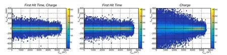
Fig.2 (Color online)The distribution of δZ as a function of the cubic radius r3.The left plot corresponds to Case A,for which both charge and FHT information was used.The middle plot corresponds to Case B with FHT information only. The right plot corresponds to Case C with charge information only. The black curve in each plot demonstrates the vertex bias, which is near 0 in all cases

Fig.3 (Color online)Energy dependence of the vertex resolution for the three cases(Charge,FHT,FHT and Charge).The top and bottom panels correspond to the central(r3＜4000 m3)and border regions(r3＞4000 m3) of the detector, respectively

4.2 Dynode versus MCP

Similar to the charge vs.time comparison,another issue is how the two types of PMTs contribute to the vertex reconstruction. To address this question, vertex reconstruction was performed using different types of PMTs, as indicated below. The same data samples and CNN model were used again;here,the inputs to the CNN included both the FHT and charge images,and the CNN was retrained for each case.

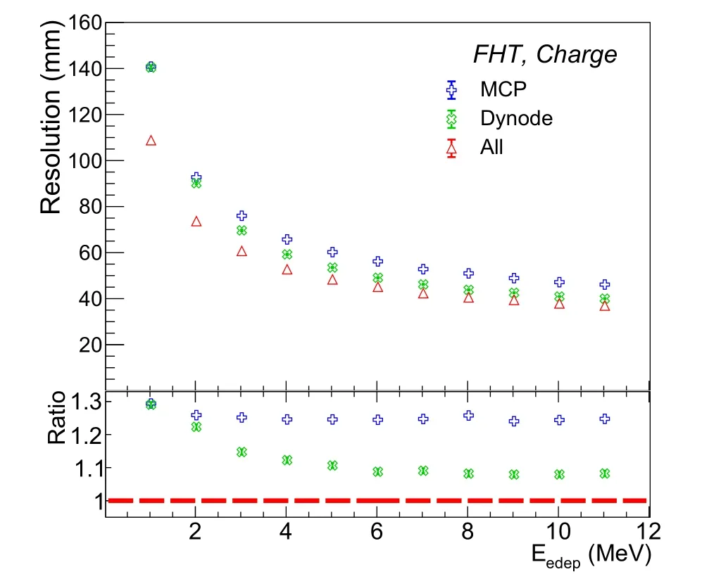
Fig. 4 Comparison of the vertex resolution among the three cases in which different types of PMTs are used.Blue indicates Case 1,where only MCP PMTs are used. Green indicates Case 2, where only Dynode PMTs are used. Red indicates Case 3, where both types of PMTs are used.The bottom panel presents the ratio of Case X/Case 3

Case 3 would typically be expected to present a significantly better vertex reconstruction performance compared to both Case 1 and Case 2, because the information of both types of PMTs were used;however,this was not the case.In the high-energy region,Case 3 had a slightly better vertex resolution than Case 2.Although,in principle,more information should provide additional constraints to help improve vertex reconstruction, the manner in which the information is utilized is also critical. Based on the aforementioned, an analogy can be made for Case 3. Considering if two cameras with significantly different resolutions were used to obtain an image of the same object; the two images would then be overlaid on top of one another to forge a combined image.A camera with a significantly bad resolution may not help in improving the quality of the combined image. On the contrary, it may make the combined image more fuzzy and possibly degrade its quality.MCP PMTs have a significantly worse time resolution compared to that of Dynode PMTs; by overlaying their FHT images, the network and result of the marginal improvement in the reconstruction performance may be confused. The number of fired PMTs is more important in the low-energy region. The use of both types of PMTs leads to a significantly better vertex resolution.

4.3 Separation of input images of PMTs

The information of both types of PMTs should be used to achieve the best vertex reconstruction performance.However, mixing the information of different types of PMTs may not be optimal, as indicated in the aforementioned section. In the traditional vertex reconstruction method presented in Ref. [14], the two types of PMTs are handled separately with different residual time PDFs owing to the varying TTS. Following the same strategy, the FHT information should be separated into two images (or channels), one for each type of the PMTs. Given that the charge resolution is also different for Dynode and MCP PMTs, the charge information can also be sufficiently segregated. To test the performance of this new strategy,several of the following scenarios were considered:

• Default case:both the charge and FHT information are mixed for the two types of PMTs, and the input to VGG-J includes one charge image plus one FHT image.

• Partially separated case: the FHT information is segregated by PMT types and there are three input images.

• Fully separated case: both the charge and FHT images are separated, resulting in four input images.

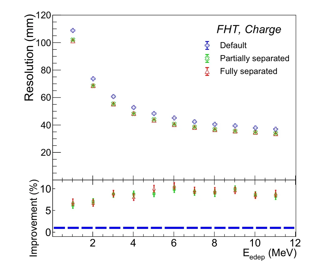
Fig.5 (Color online)Comparison of the vertex resolution among the three cases with different input images to VGG-J. Blue indicates the default case, where mixed charge and FHT images are used. Green indicates the partially separated case, where the FHT image is separated.Red indicates the fully separated case,where both FHT and charge images are segregated. The bottom panel demonstrates the improvement with respect to the default case

The VGG-J model was retrained for each case, and the performance of the vertex reconstruction was evaluated and compared. Figure 5 demonstrates a comparison of the vertex resolutions for the three cases. The red, blue, and green dots indicate the default, partially separated, and fully separated cases, respectively. Following the separation of the FHT information by PMT type, a large improvement was observed across the entire energy range with respect to the default case.For example,at 1 MeV the vertex resolution decreased from 111 mm to 102 mm, and at 11 MeV it decreased from 37 mm to 34 mm. A further separation of the charge information also leads to a better performance with respect to the partially separated case;however, it is a small improvement. For example, the vertex resolution at 1 MeV only improved from 102 mm to 101 mm. This was expected, given the large TTS difference between the two types of PMTs. On the other hand,their charge resolution was not significantly different.

For the JUNO CD, although the small PMTs were not included in this study for simplicity, adding their information is simple for vertex reconstruction using the same strategy as indicated above. When there are multiple types of PMTs in a detector, the best strategy is to separately utilize their information, especially when the characteristics of different types of PMTs are significantly different.This is true for vertex reconstruction, as demonstrated in this study,and may be applicable to other tasks in general.By using the camera analogy,each type of the PMTs forms an independent camera or sub-detector; their images or measurements should be obtained separately and then combined to achieve an optimal performance.

5 Addition of second hit

In Ref. [17], as well as all the aforementioned studies,the inputs to the CNN models are only limited to the total charge and the first hit time of each PMT. More than one photon may hit a PMT, which is both energy- and vertexdependent. As the event energy increases, more photons are emitted; consequently, all PMTs are more likely to detect more photons. On the other hand, when an event vertex approaches the border of a detector, the PMTs near the event vertex may likely receive more photons.

Given the large number of PMTs (a total of approximately 17,600)for the JUNO CD and the rough light yield of 1300 photons per MeV,for positrons with an energy less than 11 MeV, most of the PMTs will receive zero or one photon. Approximately one-third of the fired PMTs will detect more than one photon on average for all the events in the training datasets,as shown in Fig. 6.The fraction of fired PMTs that detect three or more photons drops sharply because the number of detected photons for each PMT obeys a Poisson distribution with small mean values.

In principle, all the later photon hits of PMTs also contain information regarding the event vertex. However,we only consider the second hit time(SHT)of PMTs in this study. If the addition of SHT does not improve the vertex reconstruction,it is unnecessary to include the third or later hits because their fraction is even smaller.

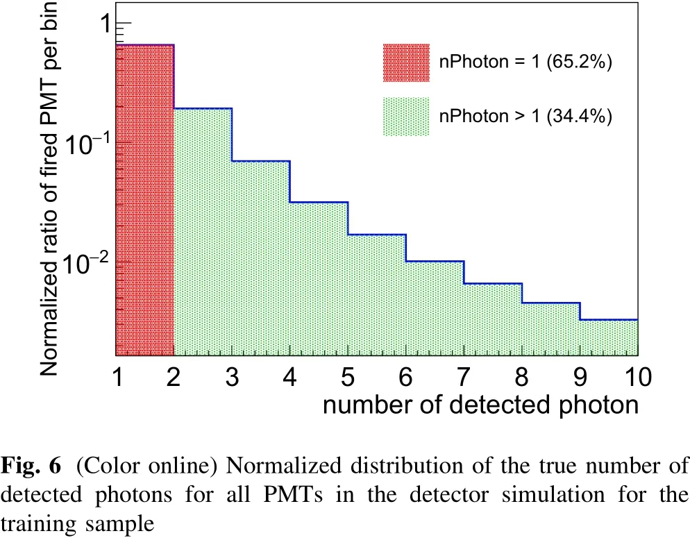
Fig. 6 (Color online) Normalized distribution of the true number of detected photons for all PMTs in the detector simulation for the training sample

5.1 Ideal case without TTS and dark noise

We start from the ideal case in which electronic effects,such as PMT TTS and dark noise are turned off. In this scenario,the two types of PMTs can be treated identically.Figure 7 demonstrates the PMT images for a positron with E=8.25 MeV and r=15.38 m in the JUNO CD in an ideal case.

Fig. 8 Comparison of the vertex resolution with and without using the SHT information in an ideal case, indicated by the red and blue dots, respectively. The bottom panel demonstrates the improvement by adding SHT, which is more pronounced as the energy increases

The left, middle, and right plots correspond to the charge, FHT, and SHT images, respectively. The projection of PMTs onto the 2D plane is the same as that shown in Fig. 1.Similar patterns in the FHT and SHT images are observed upon comparison; PMTs closer to the vertex in the FHT images are more likely to detect two or more photons and contribute to the SHT image.Presumably, the SHT information can add additional constraints on the event vertex.This can easily be verified by adding an SHT image to the VGG-J model. The reconstruction results are shown in Fig. 8, which are indicated by the red dots. The reconstruction results obtained without using the SHT image are indicated by the blue dots for comparison. In general,adding SHT improves the vertex resolution,which becomes more pronounced as the energy increases. At 1 MeV, the vertex resolution improved by approximately 1.6%,from 62 mm to 61 mm,after adding the SHT image,whereas at 11 MeV it improved by approximately 4.3%,from 23 mm to 22 mm. This is consistent with our expectation because the fraction of PMTs with SHT increases as the energy increases.

5.2 Realistic case with TTS and dark noise

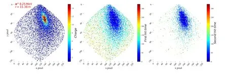
Fig.7 (Color online)Images of PMT charge and time information for a positron with E=8.25 MeV and r=15.38 m in the JUNO CD.The left,middle,and right plots demonstrate the charge,FHT,and SHT images,respectively.The photon counting time window is 1250 ns for the PMTs

In the previous section, we demonstrated that the SHT information is also useful for vertex reconstruction in an ideal scenario. In reality, the TTS and dark noise of PMTs must be considered; in Ref. [14], their impact on vertex reconstruction was exclusively studied. TTS has a dominant effect because it largely degrades the resolution of FHT. On the other hand, the contribution of PMT dark noise on the FHT is small if the rate is not too high. Thus,its impact on vertex reconstruction is relatively small in Ref. [14], where only FHT was used. Because PMT dark noise occurs randomly with respect to time, it does not contain information regarding the event vertex. These additional PMT hits from the dark noise contaminate the real photon hits and should be removed. However, discriminating all dark noise hits from real photon hits is challenging, and is beyond the scope of this study. For photons originating from the same particle and arriving at the same PMT, the corresponding PMT hits have a strong temporal correlation. This correlation can be used to partially remove the dark noise contribution, particularly for later hits. The difference between FHT and SHT was required to be less than 300 ns.This simple cut on the SHT was optimized to retain 98.9%of the real photon hits,while 48% of the dark noise hits were rejected for SHT. After applying this cut, the average fraction of the fired PMTs with SHT for all the events in the training dataset decreased from approximately 36.3% to 33.8%, which is close to the 33.3%in the ideal case without dark noise.Meanwhile,for the PMTs with SHT, the fraction of PMTs containing dark noise hits decreased from approximately 11.3% to 4.4%,similar to 4.9% for PMTs with FHT.

Fig. 9 Comparison of the vertex resolution with and without using the SHT information in a realistic case, which is indicated by the red and blue dots, respectively. The bottom panel demonstrates the improvement by adding SHT,which is approximately 1%in this case

Given that TTS is not zero in a realistic case, the information of the two types of PMTs needs to be separated to achieve the best performance, as shown in Sect. 4.3. In addition to the charge and FHT images of both types of PMTs, two additional SHT images were also fed into VGG-J, accounting for six images in total. Figure 9 compares the vertex resolution with and without the use of SHT information in a realistic case. The red dots indicate the fully separated case in Sect. 4.3, where four images were used, while the blue dots indicate the case where six images were used. Similar to the ideal case, adding SHT improves the vertex resolution in a realistic case.However,the improvement is not as prominent as that in an ideal case, which is mainly due to the degradation of the PMT time resolution caused by TTS.

Based on studies regarding both ideal and realistic cases,it is clear that SHT can improve the performance of vertex reconstruction.The time resolution of PMTs is an essential factor. For any future similar detectors, we should attempt to reduce the TTS of PMTs. We also verified that by adding SHT, the improvement was similar in the central and border regions for both cases. It is also noteworthy to consider that both the charge and time information were reconstructed from PMT waveforms. This process introduces additional uncertainties in both charge and time.Thus, we also need to develop a better waveform reconstruction method to mitigate its impact on both the charge and time resolution of PMTs.Later hits may also be useful,provided that they can be sufficiently identified and reconstructed, which tends to be difficult especially when they overlap with one another.

6 Performance summary and discussion

Two optimization methods for machine learning-based vertex reconstruction have been analyzed in this study;namely,separation of the PMT information by PMT type in Sect. 4, and addition of the SHT information in Sect. 5.The improvement in the vertex resolution is demonstrated in Figs. 5 and 9.

For convenience,Table 3 summarizes the results at 1,5 and 11 MeV. A default case without optimization is also shown for comparison.Separation of the PMT information by PMT type leads to a 10% improvement with respect to the default case. The further addition of SHT information results in another 1% improvement.

For machine learning-based vertex reconstruction, there are a few remaining aspects that need to be further investigated. First, it is a continuous process for particles to deposit energy in the LS and emit photons, which resembles a video rather than an image.The use of this temporal information may pose new challenges. Meanwhile, JUNO CD is a spherical detector, and any projection of PMTs on the surface of a sphere to a 2D plane usually causes deformation and loss of symmetry and continuity.We were able to borrow astrophysical tools to handle sphericalimages. Third, the robustness of machine learning techniques has to be verified, especially when there are discrepancies between the training and evaluating datasets,or between the Monte Carlo simulation and real data.Another issue is determining the uncertainty of the machine learning-based method. Lastly, we also need to compare the precision of different vertex reconstruction algorithms with real data. One possible approach is to use calibration data with known vertex information.Another approach is to rely on a Monte Carlo simulation after being tuned to real data.Moreover, an alternative option is using reinforcement learning with hybrid training samples of calibration and simulation data. By addressing these topics in the future,we aim to achieve the best vertex reconstruction for large LS detectors with multiple types of PMTs and consequently enhance the detector performance to increase the physical potential of new discoveries.

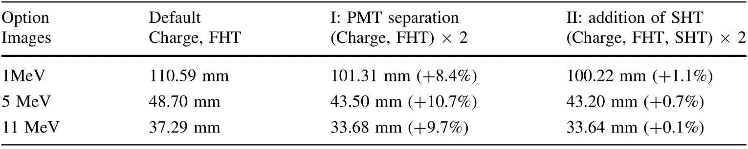
Table 3 Comparison of the vertex resolution with different options of input images

7 Conclusion

A high-precision vertex resolution is essential for large liquid scintillator detectors, such as JUNO. There are several studies [2, 14, 35] regarding vertex reconstruction using traditional methods for liquid scintillator detectors,whereas the novel idea of vertex reconstruction with machine learning techniques has only been recently applied to JUNO for the first time [17]. In this study, we continue to improve the performance of machine learning-based vertex reconstruction and focus on the optimization of the input images to the CNN model. Owing to the different characteristics of various types of PMTs, their information is separated rather than mixed.Moreover,in addition to the FHT information of PMTs, the SHT information was also used. The separation of the two types of PMTs led to a noticeable improvement in the vertex resolution of approximately 10% on average across the energy range of[1, 10] MeV. The further addition of SHT resulted in an improvement of approximately 1% on average. These two optimization methods appear to be relatively simple;however, they can be used as general guidelines for other detectors with multiple types of PMTs.

AcknowledgementsWe would like to thank the Computing Center of IHEP for providing the GPU clusters.

Author contributionsAll authors contributed to the study conception and design. Material preparation, data collection and analysis were performed by Zi-Yuan Li and Zhen Qian. The first draft of the manuscript was written by Zheng-Yun You, Yu-Mei Zhang and Wu-Ming Luo. All authors commented on previous versions of the manuscript. All authors read and approved the final manuscript.