Study on analytical noise propagation in convolutional neural network methods used in computed tomography imaging

Xiao-Yue Guo• Li Zhang • Yu-Xiang Xing

Abstract Neural network methods have recently emerged as a hot topic in computed tomography (CT) imaging owing to their powerful fitting ability; however, their potential applications still need to be carefully studied because their results are often difficult to interpret and are ambiguous in generalizability.Thus,quality assessments of the results obtained from a neural network are necessary to evaluate the neural network.Assessing the image quality of neural networks using traditional objective measurements is not appropriate because neural networks are nonstationary and nonlinear. In contrast, subjective assessments are trustworthy, although they are time- and energy-consuming for radiologists. Model observers that mimic subjective assessment require the mean and covariance of images, which are calculated from numerous image samples; however, this has not yet been applied to the evaluation of neural networks. In this study, we propose an analytical method for noise propagation from a single projection to efficiently evaluate convolutional neural networks (CNNs) in the CT imaging field. We propagate noise through nonlinear layers in a CNN using the Taylor expansion. Nesting of the linear and nonlinear layer noise propagation constitutes the covariance estimation of the CNN. A commonly used U-net structure is adopted for validation.The results reveal that the covariance estimation obtained from the proposed analytical method agrees well with that obtained from the image samples for different phantoms, noise levels, and activation functions, demonstrating that propagating noise from only a single projection is feasible for CNN methods in CT reconstruction. In addition, we use covariance estimation to provide three measurements for the qualitative and quantitative performance evaluation of U-net. The results indicate that the network cannot be applied to projections with high noise levels and possesses limitations in terms of efficiency for processing low-noise projections. U-net is more effective in improving the image quality of smooth regions compared with that of the edge. LeakyReLU outperforms Swish in terms of noise reduction.

Keywords Noise propagation ∙Convolutional neural network ∙Image quality assessment

1 Introduction

In recent years, neural networks have been applied in computed tomography (CT) imaging. Several studies on the applications of such networks have been published,and their potential in solving several problems in the field of CT imaging has been extensively evaluated.Such networks have been used in applications such as spectral distortion correction [1, 2] for photon-counting X-ray CT, dual-domain learning for two-dimensional [3, 4] and three-dimensional [5–7] low-dose CT reconstruction, sparse-view[8] and limited-angle [9] CT reconstruction, noise suppression in the sinogram domain [10] and image domain[11], dual-energy imaging with energy-integrating detectors [12] and photon-counting detectors [13], and CT artifact reduction[14,15].However,neural networks have not yet been widely used in practice owing to their confidence scores. Hence, researchers have adopted objective and subjective image quality assessments to evaluate the feasibility of using neural networks in CT imaging[16,17].However, traditional metrics are preferred for objective assessments. The commonly used contrast-to-noise ratio measures the region of interest (ROI) clarity, signal-tonoise ratio measures the noise level,noise power spectrum(NPS) measures the noise correlation, and modulation transfer function measures the spatial frequency [18, 19].Neural networks are normally nonlinear,nonstationary,and unexplainable; however, to the best of our knowledge,limited research on theoretically tractable methods has been conducted.

Subjective assessments are commonly used in the field of CT imaging. Radiologists are invited to observe and score images obtained from various methods [20, 21].Because subjective assessments are time-consuming and laborious, researchers study model observers to simulate the evaluation behavior of radiologists. The assessment of image quality carried out by a radiologist,that is,a human observer is modeled as a classification problem solved by hypothesis testing. The likelihood ratio is used as the decision variable to obtain an ideal observer(IO).Because the IO is intractable, a linear approximation of the IO is assumed to obtain a Hotelling observer (HO). Combining the human-eye model with HO, researchers have obtained the most widely used channelized Hotelling observer(CHO) [22]. The CHO agrees well with human observers[23, 24]; however, it requires knowledge of the image mean and covariance.Recently,neural networks have been introduced to explore nonlinear model observers that enable better approximation of the human observer or better detectability for auxiliary diagnoses [25–27]. However, these methods only target traditional reconstruction methods [28, 29]. The application of these methods to neural network reconstruction has not yet been explored.

Noise propagation through a reconstruction neural network is necessary for assessing the performance of the network. Covariance prediction can reveal the uncertainty in inference, thus providing a safer answer to the CT reconstruction problem. Furthermore, it can be used in the calculation of model observers and subjective assessments.

The covariance estimation of neural-network outputs is currently of significant interest. Abdelaziz et al. [30]studied the uncertainty propagation of deep neural networks for automatic speech recognition with the assumption that the output was Gaussian. Lee et al. [31] used a Gaussian process equivalent to a deep fully connected neural network to obtain an exact Bayesian inference under the assumption that the parameters and layer outputs follow an independent and identical distribution.Tanno et al.[32]simultaneously estimated the mean and covariance of highresolution outputs from low-resolution magnetic resonance images based on the assumption of a Gaussian distribution.However, for CT imaging, covariance estimation of the neural network output has not yet been studied.

In this study, we propose a new analytical noise propagation method, that is,covariance estimation, particularly for a convolutional neural network (CNN) in CT imaging of noisy projections. With a trained CNN ready for inference, we propagate the noise layer by layer. For linear layers, the output covariance can be calculated accurately.For nonlinear activation layers, we perform a Taylor expansion to obtain a linear approximation, which enables linear propagation of noise through the nonlinear layers.Because a CNN is a stack of linear and nonlinear layers,its covariance estimation is a combination of layer noise propagations. We validate the results of the covariance estimation method by comparing the results with those of statistical estimations using noisy projection and reconstruction samples with different phantoms, noise levels,and activation functions.

2 Methods

2.1 Physical model for CT imaging

A simple model for data acquisition in a CT scan is formulated as

where φldenotes the operation function of one layer,and Φ denotes the overall function of the neural network. Evidently, the noise in p will result in a noisy μ, even though several networks are used to reduce noise. We discovered that the noise propagation through φl’s to output μ can be studied step-by-step if a network model is ready to serve for inference, that is, network parameters are set. The key lies in sorting out the covariance estimation through the five basic layers constituting the entire CNN.

2.2 Covariance propagation through basic layers of a CNN

Let vector x ∊RM×1be an arbitrary layer input, and let y be the corresponding layer output. This section presents the covariance estimation of y from x.

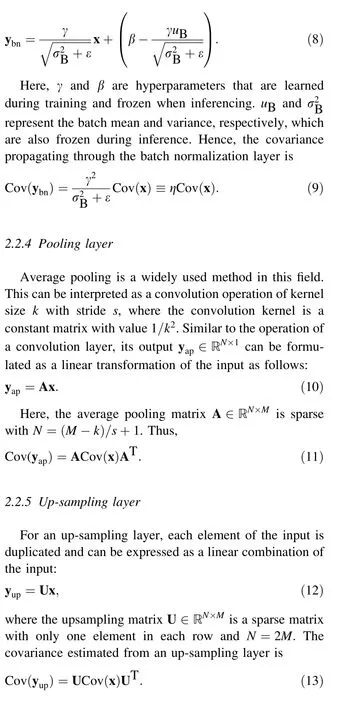
2.2.3 Batch normalization layer

For a batch normalization layer, the input is normalized as

2.3 Example: U-net

We adopt a commonly used U-net structure to denoise the projection, followed by reconstruction with the filter back projection (FBP) method:

Here, O represents the linear FBP operator. p ∊RM×1denotes an input projection, and μ ∊RN×1represents the corresponding reconstruction. The reconstructionflowchart is illustrated in Fig. 1. A concatenate layer and residual layer are included in U-net. The concatenated layer merges the feature map in the 1st layer to the 6th layer,and the residual layer adds the input projection to the 9th layer to obtain the output projection.

Fig. 1 (Color online) U-net structure for CT reconstruction.The projection is first filtered by U-net and then reconstructed by FBP. Two activation functions:①LeakyReLU and ②Swish,are applied to U-net

We iteratively estimate the covariance of reconstruction predicted from the trained U-net:

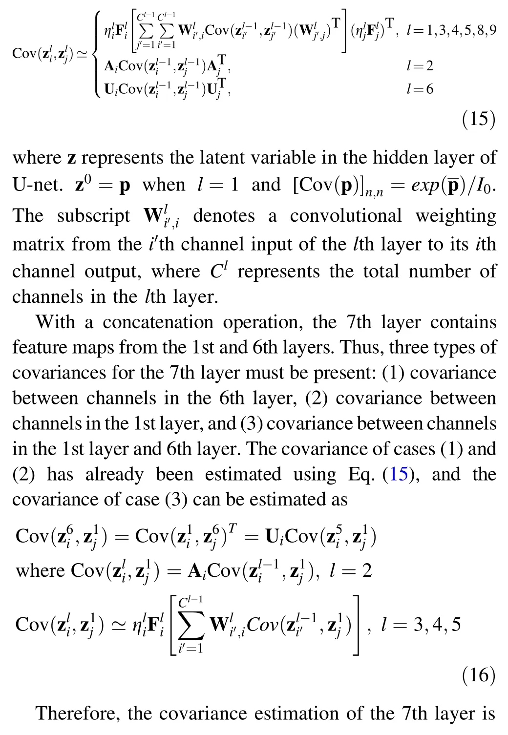
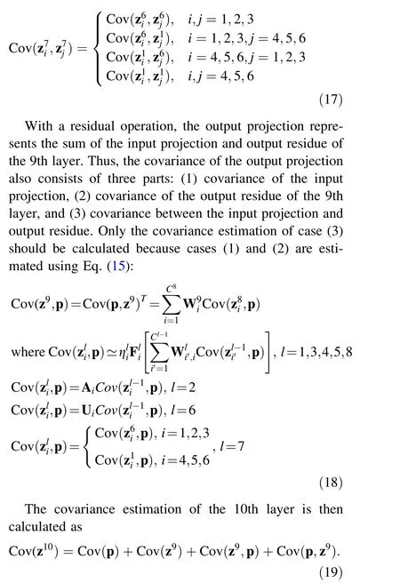
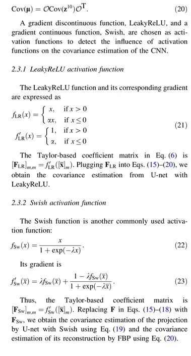
Combining Eqs. (15)–(19), we obtain the final covariance estimation of the reconstruction:

3 Experiments

The projectiondatausedfor trainingare generatedfromthe Grand Challenge dataset of the Mayo Clinic. We randomly choose a reconstruction dataset of one patient and select various ROIs with sizes of 128 × 128 pixels as phantoms.Geometrical parameters of the simulated system are listed in Table 1. By setting the number of incident photons to I0=104,we add Poisson noise to the noise-free projections simulated from phantoms to obtain noisy projections.

Using noise-free projections as labels and noisy projections as inputs, we train U-net by minimizing an L2 norm loss function between labels and outputs.In addition,we fix the hyper-parameter α=0∙1 for LeakyReLU and λ=0∙5 for Swish. We simulate 1792 noisy projections for the study. The dataset is randomly split into a training set and a validation set, where 80% of the dataset represents the training set and 20% represents the validation set. We train the network with Keras on a GPU RTX8000 of 48G.The loss function of U-net with LeakyReLU and Swish decreases to approximately 10-4during converging. Furthermore,we randomly split the dataset into 5 folds to run a fivefold cross validation on the trained network. The average loss in the fivefold cross validation is also approximately 10-4, which is similar to the loss of the trained network. Thus, the dataset is sufficient for training the small-size U-net in Fig. 1, and the trained network is stable.

Table 1 System geometry of simulation experiments

Noisy projections used for inference are generated from another patient dataset in the same manner. We generate noisy projections of different phantoms and noise levels to validate the proposed analytical noise propagation method and analyze the performance of U-net using the analytically estimated covariance. Information on the noisy projections generated for prediction is presented in Table 2.Note that the number of incident photons increases linearly from 103to 5.05 × 104. The reconstruction of both phantoms using I0=104is illustrated in Fig. 2.

In addition, we conduct a practical experiment to validate our proposed method. The experimental platform and phantom are presented in Fig. 3. The scanning parameters are presented in Table 3. We repeat the scan 450 times at each angle and acquire projection data of 360 views using 2π. Considering the computational cost, every four pixels of the detector are binned into one to obtain a projection with a smaller size.

Covariance estimation from a statistical method is used as a reference in this study.

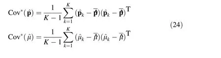
Table 2 Information on the noisy projections generated for inference

Fig. 2 Denoised projections of a test phantom A and b test phantom B for I0 =104 obtained from U-net and their reconstructions obtained from FBP

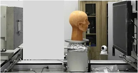
Fig. 3 (Color online) Experimental platform and phantom

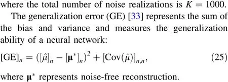
Table 3 Scanning parameters of the practical experiment

Here, μ=O(p) and Cov(μ)=OCov(p)OT, according to Eq. (20). We choose one low-attenuation point and one high-attenuation point in test phantom B to present the trend of GE with the noise level;the two points are marked by red dots in Fig. 2b.

We also calculate the NPS to analyze the noise spatial correlation of U-net in the Fourier domain:

where F denotes the Fourier transform operator.

4 Experimental results

Because the linear approximation of nonlinear activation functions requires the mean of the input in Eq. (6),we only use one noise realization as the mean of the input to analytically estimate the covariance of the projection acquired by U-net and its corresponding reconstruction by FBP.

4.1 Validation of the proposed analytical covariance estimation method for U-net

For test phantom A, the variance of the projections obtained by U-net is illustrated in Fig. 4a, and its covariance at the center of the projections is presented in Fig. 4b.The results reveal that the variance estimation is in agreement with the reference for both the activation functions. The error between the variance estimation and reference is not significant compared with the variance itself. We observe that the variance obtained from LeakyReLU varies sharply when approaching the boundary,whereas that from Swish changes smoothly. Meanwhile,the covariance estimation also agrees with the reference,where the error is primarily statistical. The shape of the covariance from the two activation functions is quite different; it is circular for LeakyReLU and elliptical for Swish. For test phantom B, good agreement can still be observed between the variance estimation and reference(as shown in Fig. 4c). Sharp changes also occur near the boundary in the projection variance from LeakyReLU. As shown in Fig. 4d, the covariance estimation for both activation functions is in agreement with the reference.

The variance and covariance of the reconstructions obtained by FBP from projections denoised by U-net are presented in Fig. 5. For both phantoms and activation functions, the variance estimation of the reconstructions agrees with the reference because FBP is linear. Meanwhile, the error that propagates through the FBP is not a concern. We discover that the central areas of variance from the two activation functions have different appearances. The central area appears dark for LeakyReLU and bright for Swish in the same display window. The covariance estimation is yet again in agreement with the reference, leaving only statistical noise in the error map.

The profiles of the variance and covariance for the projections and reconstructions are plotted in Fig. 6. For both phantoms and activation functions, the profiles of the variance and covariance estimations match those of the references. As shown in Fig. 6a1, c1, the profile of the projection variance from Swish appears smooth, whereas that from LeakyReLU appears sharp. The profile of covariance (as shown in Fig. 6b1 and d1) from Swish demonstrates a larger spread, whereas that from LeakyReLU exhibits sharper changes. For the profiles of the reconstruction variance, displayed in Fig. 6a2 and c2, we discover that the noise from LeakyReLU is lower than that from Swish. The variance gradually decreases from the edge of the field of view (FOV) to its center for LeakyReLU, whereas it demonstrates an opposite behavior for Swish.Although the values of the projection covariance are close, the absolute value of the reconstruction covariance from LeakyReLU is much smaller than that from Swish;this demonstrates that the covariance from Swish is more structurally related and difficult to deal with.

In addition, we estimate the variance of the projections obtained by U-net with LeakyReLU under different noise levels for test phantom B.As shown in Fig. 7,the variance estimation agrees with the reference for different noise levels. Although the error between the variance estimation and reference increases with the noise level, it is still insignificant compared with its corresponding variance.

The noise estimation of U-net with LeakyReLU in the practical experiment is illustrated in Fig. 8. It is apparent that both the variance and covariance estimations from the analytical method agree well with the references, which strongly demonstrates the feasibility of the proposed analytical noise propagation method in practical usage.

4.2 Performance analysis with analytical covariance

Pixel-wise GE maps for test phantom B are illustrated in Fig. 9.For both activation functions,GE increases for each pixel with increasing noise levels, which indicates that Unet is inapplicable for highly noisy projections. When I0increases to a certain number, the decrease in GE is not significant. The GE in the smooth region is smaller than that at the edge when the number of incident photons increases to 3∙25×104, indicating that U-net is more effective in smooth regions. Compared with the GE for LeakyReLU,the GE for Swish is relatively large in smooth regions, whereas it is almost the same at the edge.

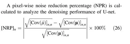
Further, noise reduction percentage (NRPs)are listed in Table 4.For both activation functions,the increase in NRPfrom I0=103to I0=5∙5×103is approximately 20%,and this increase quickly slows to approximately 5% or less.For both low- and high-attenuation points, the noise reduction effect of LeakyReLU is stronger than that of Swish at various noise levels. The NRP of LeakyReLU is approximately 10% higher than that of Swish, particularly for the low-attenuation point at I0=103,and the difference decreases to approximately 1% for a low noise level with I0=5∙05×104. For the high-attenuation point, the difference in the NRP for both activation functions is smaller than 3% and becomes even smaller when the number of incident photons increases. The NRPs at both points for LeakyReLU are comparable, which suggests that LeakyReLU treats low- and high-attenuation areas equally during noise suppression. The NRP at the low-attenuation point for Swish is slightly smaller than that at the highattenuation point; however, the difference between the NRPs at the low- and high-attenuation points gradually reduces to approximately 1% with decreasing noise levels.

Fig. 4 Variance of the projections obtained from U-net and its covariance at the center of projections when I0 =104.a and c projection variance of phantom A and B used for testing, respectively. b and d corresponding covariance at the center of the projection

The NPS at the center of the reconstruction is illustrated in Fig. 10.For each noise level,the NPS at the center of the reconstruction from both activation functions decreases as 103increases to 5∙05×104and drops by approximately an order of magnitude from 103to 5∙5×103. The NPS from LeakyReLU first increases to a maximum and then decreases as the frequency increases, whereas that from Swish continues to increase with increasing frequency.Both LeakyReLU and Swish exhibit similar NPS shapes at low frequencies, indicating that their performance in dealing with low-frequency noise is comparable.The highfrequency noise in the NPS from LeakyReLU gradually reduces; however, it increases considerably for Swish,suggesting that more structures are present in the reconstruction noise propagated through U-net with Swish.

5 Discussion and conclusion

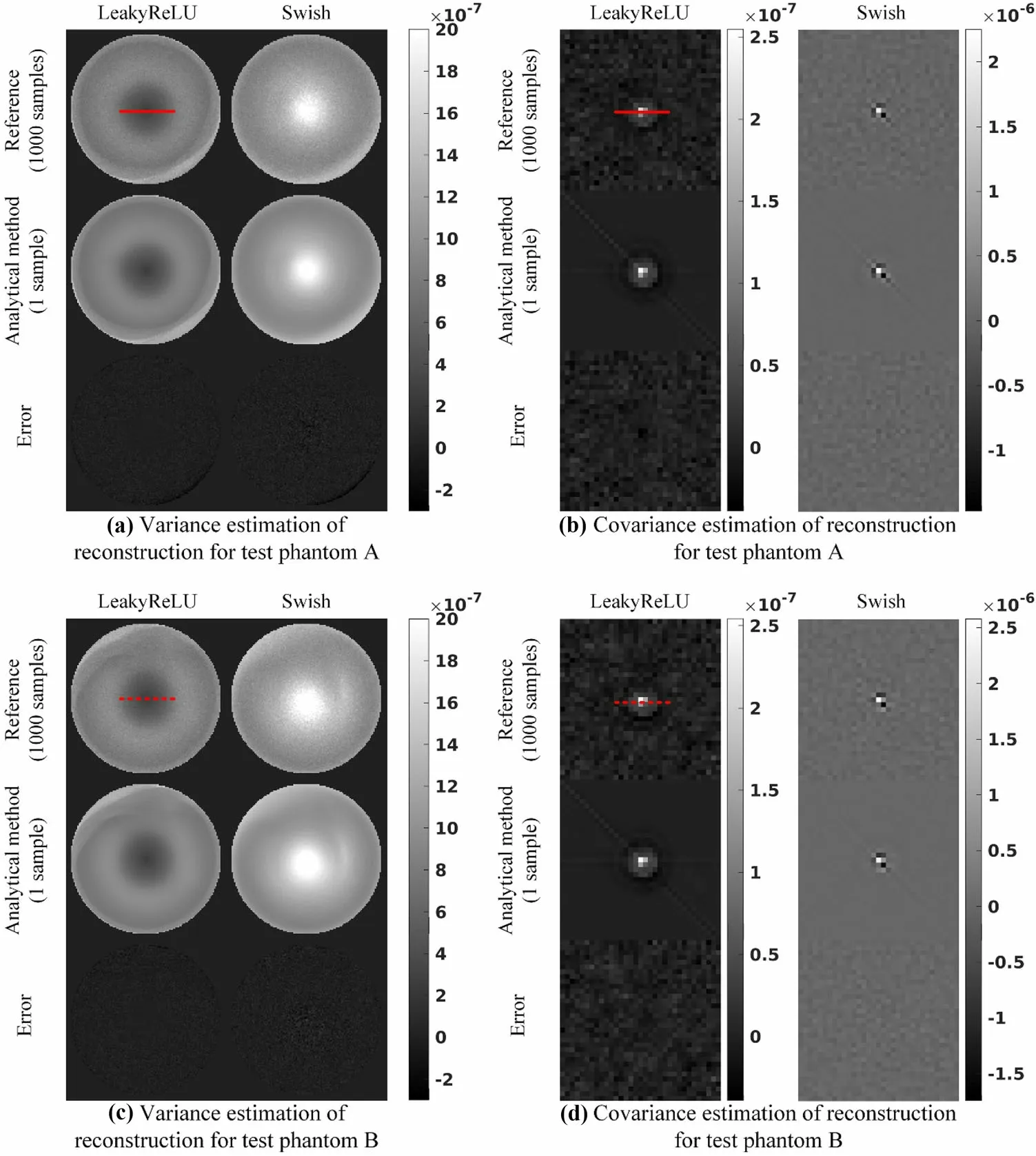
Fig. 5 Variance of the reconstructions by FBP from projections obtained from U-net and its corresponding covariance at the center of the reconstructions for I0 =104.a the reconstruction variance of test phantom A and b its covariance at the center of reconstructions. c the reconstruction variance of test phantom B,and d its covariance at the center of reconstructions

In this study,an analytical noise propagation method for CNNs in CT imaging is proposed.The five basic layers that comprise a typical CNN include the convolution,nonlinear activation, batch normalization, average pooling, and upsampling layers. Except for the nonlinear activation layer,the other four layers are all linear, which simplifies the estimation of the covariance of their output by linear propagation. The 1st order Taylor expansion is used to obtain the linear approximation of the nonlinear activation layer for linear propagation of noise. By integrating the noise propagation of both linear and nonlinear layers in the CNN, we can estimate the covariance of reconstruction from the projection in a step-by-step manner.

The results indicate that the covariance estimated by the proposed analytical method agrees well with that estimated by the statistical method, regardless of phantoms, noise levels, and activation functions. We demonstrate that it is feasible to propagate noise from only a single projection to image reconstructed from CNN. The covariance of the projection obtained from U-net with the gradient continuous activation function Swish is smooth,whereas that with the discontinuous gradient activation function LeakyReLU exhibits sharp changes near the boundary.The noise in the reconstruction from LeakyReLU is smaller than that in Swish.They demonstrate opposite performances,where the variance from Swish gradually decreases from the FOV edge to its center. Therefore, LeakyReLU and Swish are completely different in terms of noise suppression. The covariance for Swish spreads wider than that for LeakyReLU, which indicates that Swish uses the information of more neighborhood pixels in denoising.

We further qualitatively and quantitatively evaluate network performance from three aspects. The GE, which contains bias and variance, is a tradeoff between the accuracy and noise of the network output and measures the generalization of the neural network. Trained with data under the condition of I0=104,the network fails to reduce the GE for projections with lower incident photons, which renders it unacceptable for application in projection denoising with high noise levels. This also limits its application to projections with lower noise when I0increases to a certain number because the improvement inGE is trivial. A pixel-wise NRP is defined to measure the denoising ability of the network. The effect of noise suppression is strong only when the noise level is sufficiently high; otherwise, it quickly weakens as the noise level decreases. An evident drop in GE can be observed in smooth regions but not at the edge when the number of incident photons increases, although the NPRs for smooth regions and the edge are the same.Therefore,the accuracy of the smooth regions is higher than that of the edges. In addition, the spatial correlation of noise is analyzed using the NPS. Consequently, it is discovered that there is no significant difference in NPS between LeakyReLU and Swish at low frequencies. However, the NPS at high frequencies is completely opposite for these two activation functions,where it weakens with increasing frequencies for LeakyReLU. The variance in projection denoised by the two activation functions is comparable; however, the NRP of the reconstruction from LeakyReLU is larger than that of Swish, and the NPS of the reconstruction from Swish increases as the frequency increases. Thus, both activation functions demonstrate comparable performance in projection denoising; however, their different noise distributions lead to different effects of noise suppression in reconstruction. Swish utilizes information from more adjacent pixels in noise reduction; therefore, its noise is too structural to be handled by FBP. The noise correlation of LeakyReLU is lower and easier to process. Therefore, the image quality of the reconstructions from LeakyReLU is better than that of Swish in terms of noise suppression.

Fig.6 (Color online)Profiles of the projection variance and covariance obtained from U-net,and profiles of its reconstruction variance and covariance obtained from FBP for I0 =104.a1–d1 profiles of the projection variance and covariance:a profiles of the variance marked by a red solid line in Fig. 3a for test phantom A, and b1 profiles of its covariance marked by a red solid line in Fig. 3b, c profiles of the variance marked by a red dashed line in Fig. 3c for test phantom B, and d1 profiles of its covariance marked by a red dashed line in Fig. 3d. a2–d2 profiles of the reconstruction variance and covariance: a2 profiles of the variance marked by a red solid line in Fig. 4a for test phantom A, and b2 profiles of its covariance marked by a red solid line in Fig. 4b, c2 profiles of the variance marked by a red dashed line in Fig. 4c,and d2 profiles of its covariance marked by a red dashed line in Fig. 4d

Fig. 7 Variance of projections obtained from U-net with LeakyReLU under different noise levels for test phantom B

In summary, the proposed analytical noise propagation method is capable of providing a reasonable pixel-wise noise property estimation from only a single sample,whereas other noise estimation methods cannot present comparable performance under the same conditions. Ourproposed method can be applied to any inference-ready CNN with a fixed structure and weight for noise estimation.Because the convolution, batch normalization, average pooling, and up-sampling operations are all linear, and the nonlinear activation function is linearly approximated, the noise of the network input propagates linearly in the network. Evidently, the error in the noise estimation of the network output results from the linear approximation of the nonlinear activation function. Two activation functions,LeakyReLU and Swish, are validated in this study; hence,the proposed method is applicable to any network with these two activation functions, regardless of the network structure. Moreover, the noise property estimation of the network output can be used to evaluate the performance of the reconstruction methods. We can characterize noise features based on pixel-by-pixel noise estimation, which also enables us to analyze the spatial correlation and structural properties of noise. The experimental results reveal the significant value of this method in evaluating the output from CNN methods. In future studies, we aim to study the application of covariance estimation to a model observer for subjective image quality assessment. However, the computational cost is expected to increase with increasing network complexity and dimensions. Hence,efficient noise propagation methods for complex and highdimensional networks must be studied.

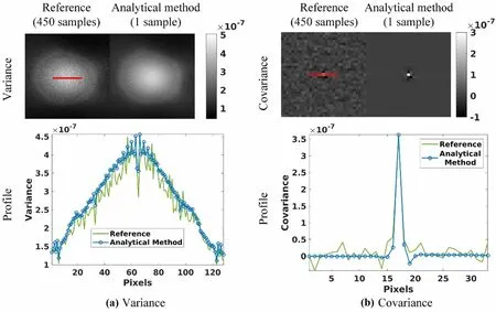
Fig. 8 (Color online) Noise properties of reconstruction from the projection produced by U-net with LeakyReLU for the practical experiment. a The variance and profiles are marked by the red solid line, and b the covariance at the center of the reconstruction and the profiles are marked by the red solid line

Fig. 9 GE maps of U-net with varying noise levels for test phantom B

Table 4 NRPs of U-net with varying noise levels.Point ①represents the low-attenuating point,and point ②indicates the high-attenuating point.Both points are marked by red dots in Fig. 2(b)

Fig. 10 (Color online) NPS at the center of reconstructions varying with the number of incident photons. a NPS of reconstructions with varying noise levels. b–d NPS profiles of different noise levels: b NPS profiles at I0 =103, c NPS profiles at I0 =5∙5×103 and 104,and d NPS profiles at I0 =3∙25×104 and 5∙05×104

Author contributions All authors contributed to the study conception and design. Material preparation, data collection and analysis were performed by XYG, LZ, and YXX. The first draft of the manuscript was written by XYG and all authors commented on previous versions of the manuscript. All authors read and approved the final manuscript.