Finite-Time Distributed Identification for Nonlinear Interconnected Systems
2022-07-18FarzanehTatariHamidrezaModaresChristosPanayiotouandMariosPolycarpou
Farzaneh Tatari, Hamidreza Modares,,, Christos Panayiotou, and Marios Polycarpou,,
Abstract—In this paper, a novel finite-time distributed identification method is introduced for nonlinear interconnected systems. A distributed concurrent learning-based discontinuous gradient descent update law is presented to learn uncertain interconnected subsystems’ dynamics. The concurrent learning approach continually minimizes the identification error for a batch of previously recorded data collected from each subsystem as well as its neighboring subsystems. The state information of neighboring interconnected subsystems is acquired through direct communication. The overall update laws for all subsystems form coupled continuous-time gradient flow dynamics for which finitetime Lyapunov stability analysis is performed. As a byproduct of this Lyapunov analysis, easy-to-check rank conditions on data stored in the distributed memories of subsystems are obtained,under which finite-time stability of the distributed identifier is guaranteed. These rank conditions replace the restrictive persistence of excitation (PE) conditions which are hard and even impossible to achieve and verify for interconnected subsystems.Finally, simulation results verify the effectiveness of the presented distributed method in comparison with the other methods.
I. INTRODUCTION
INTERCONNECTED systems are composed of several(possibly heterogeneous) physically connected subsystems influencing each other’s behavior. Numerous engineering systems with practical relevance belong to this class of systems, including intelligent buildings, power systems,transportation infrastructure and urban traffic systems.Typically, distributed control and monitoring methods for interconnected systems rely on high-fidelity models of the subsystems. Designing controllers based on coarse dynamic models and without generalization guarantees may induce closed-loop systems with poor performance or may even result in instability. Moreover, failure in accurate and timely identification of the dynamics of a single subsystem may snowball into an entire network instability due to the physical interconnections among subsystems.
However, identifying the dynamics of interconnected systems is challenging due to the physical interconnections among the subsystems. This makes the existing system identification methods for single-agent systems not directly applicable to interconnected systems. Developing system identifiers with finite-time guarantees for interconnected systems is of utmost importance in practice, since it allows the designer to preview and quantify the identification errors. The preview and qualification of the error bounds can in turn be leveraged by the control and/or monitoring systems to avoid conservationism. Otherwise, the conservationism introduced due to slow or asymptotic convergence can degrade the interconnected system performance. This motivates the goal of this paper,which is to design an online distributed identifier for interconnected systems with finite-time convergence properties.
Different types of multi-agent systems’ learning approaches,classified as centralized, decentralized, and distributed identification methods, typically employed in control of multiagent systems [1]−[5], can be adopted to identify interconnected system dynamics. Centralized identification methods rely on the existence of a learning center that receives data from all subsystems and identifies the dynamics of the entire network. The centralized approach, however, comes at a high computation and communication cost and requires access to the global knowledge of the subsystems’ interconnection network. By contrast, in the decentralized learning, an independent identifier is allocated for every subsystem which only relies on the subsystem’s own information to identify its dynamics. Since there is no exchange of state information among the subsystems, decentralized identifiers are unable to identify the interconnection terms in the dynamics of subsystems. On the other hand, distributed learning methods can accurately identify the interconnected system dynamics by employing a local identifier for every subsystem while allowing it to communicate its state information with its neighboring interconnected identifiers. In contrast to the centralized method, in the distributed identification approach,no access to the global knowledge of the interconnection network is required.
The distributed identification of interconnected systems can be performed either online or offline. Generally, in offline(batch) distributed identification [6], a rich batch of data must be collected from each subsystem and its neighboring subsystems to provide high confidence generalization guarantees across the entire operating regimes of subsystems [7]−[11].In the batch learning, finite-time or non-asymptotic convergence refers to generalized guarantees provided by finite number of samples satisfying the condition of independent and identically distributed (i.i.d) which is difficult to obtain and hard to verify in closed-loop interconnected systems. On the other hand, online distributed identification, which is the problem of interest in this paper, uses online data from each subsystem and its neighboring subsystems to learn the dynamics of interconnected system in real time. Nevertheless,standard approaches for online identification require the restrictive persistence of excitation (PE) condition [12], [13]to ensure generalization and exact parameter convergence.This includes online identification of interconnected systems using both decentralized [14], [15] and distributed [16], [17]learning approaches. The PE condition, however, is hard to achieve and to verify online and its satisfaction is much more challenging for interconnected subsystems compared to single-agent systems. This is because the regressor’s PE condition for a subsystem not only depends on the richness of its own data but also the interactive data collected from its interaction with its neighboring subsystems.
To satisfy the regressor’s PE condition in interconnected systems, all subsystems must synchronously inject probing noises into their control systems to excite their dynamics and consequently to produce rich data for the entire network of subsystems. Designing such a probing noise for every subsystem to collectively satisfy the regressors’ PE conditions for all subsystems while not jeopardizing the overall system stability is a daunting challenge due to the subsystems’interconnectivity: the probing noise can snowball in the entire network and lead to the system instability. Therefore,designing an identification method for interconnected systems without requiring restrictive PE conditions, for which their satisfaction can deteriorate the system’s stability and performance, is of vital importance.
To relax the restrictive PE condition, the concurrent learning (CL) technique has been widely leveraged [18]−[31].However, existing CL results are limited to control and identification of single-agent systems. In CL methods, past recorded data are replayed along with the current stream of data in the update law to not only minimize the identification error for the current data but also for the batch of recorded data. CL methods [18]−[27] typically guarantee the asymptotic convergence of the estimated parameters. Recently, a few CL-based methods [28]−[31] provided the finite-time convergence for the estimated parameters. However, all the aforementioned finite-time approaches are dealing with identification of a single dynamic system. For interconnected systems, the identification error dynamics are only guaranteed to be locally uniformly ultimately bounded [14]−[17].
Based on the concept of finite-time stability [32], several finite-time control methods have been developed for output feedback control [33] and multi-agent system consensus [34],[35]. In finite-time control design methods, the controllers are designed to guarantee finite-time stability of the system dynamics or tracking error dynamics where either no learning is accomplished or some observers are used along with identifiers whose identification precision is not taken into account;therefore, there is no requirement on the data richness.
Moreover, several distributed asymptotic-convergent estimators have been designed in [36], [37] to estimate the system states or a specific parameter for multi-agent systems with known dynamics for which the learning objectives and therefore the rich data recording do not exist. In contrast, in the multi-agent system identification, a precise model of the system is not available and the richness of the employed data affects the identification results. For the multi-agent system identification, specifically interconnected systems, finite-time approaches are essential to assure collecting rich data to identify the system dynamics in finite time. However, finitetime identification of interconnected systems is unsettled.
This paper aims to identify the interconnected system dynamics in finite time by proposing a novel distributed discontinuous CL-based estimation law without requiring the standard regressors’ PE condition. To this end, a distributed finite-time identifier is allocated to every subsystem that leverages local communication to not only learn the subsystem’s own dynamics but also the interconnected dynamics based on its own state and input data, and its neighbors’ state information. Moreover, in order to relax the regressors’ PE condition and guarantee finite-time convergence, a discontinuous distributed CL-based gradient descent update law is presented. Using the presented update law, every local identifier minimizes the identification error at the current time based on the current stream of data from its own state and that of its neighbors as well as the identification error for data collected in a rich distributed memory. Since finite-time convergence is possible only with discontinuous or nonlipschitz dynamics [38], the discontinuous gradient flow of the identification errors for the stored samples is leveraged. The dynamics of the gradient flows are analyzed using finite-time stability and it is shown that for every subsystem an easy-toverify rank condition on the matrix containing the recorded filtered regressor data (that is used to avoid state derivative measurements) is sufficient to ensure finite-time convergence.Furthermore, joint optimization over data sampling and modeling error is possible in this framework: data optimization can be performed to optimize the spectral properties of the recorded interactive data by replacing old data with new rich data to improve the convergence speed of the modeling error. In sharp contrast, there is no mechanism in standard identification methods to optimize over data or check if the regressor’s PE condition is satisfied.
Two different cases are considered in this paper: 1)Realizable system identification for which there is a set of model parameters that can make the identification error zero.That is, the minimum functional approximation error (MFAE)is zero and is realized by an optimal set of unknown system parameters; and 2) Non-realizable system identification for which there are no model parameters that result in zero identification error. For Case 2, the subsystems have mismatch identification errors and their MFAEs are nonzero.In both cases, linearly parameterized universal approximators such as radial basis function neural networks are used to model the uncertain system functions. It is shown that under a verifiable rank condition, the proposed approach results in finite-time zero identification error for Case 1 (which is a special form of Case 2) and finite-time attractiveness to a bound near zero for Case 2.
The main contributions of this paper are as follows.
i) A novel finite-time distributed CL identification method is presented for nonlinear interconnected systems. The proposed discontinuous distributed CL estimation law ensures the finite-time convergence of the approximated parameters without requiring the regressors’ PE condition.
ii) In the proposed distributed CL, every distributed identifier leverages a local state communication with its neighboring subsystems to collect and employ a rich distributed memory to relax the regressor’s PE condition and identify its own interconnected subsystem dynamics in finite time.
iii) Based on finite-time Lyapunov analysis, when there is zero MFAE, the finite-time convergence of interconnected system parameters is ensured through rigorous proofs. For the case with non-zero MFAE, finite-time attractiveness of the interconnected system parameters’ estimation error is guaranteed.
iv) Finally, the upper bounds of the settling-time functions for the finite convergence time are provided as a function of distributed memory data richness.Notation:The network of subsystems in an interconnected system is shown by a bidirectional graphG(V,Σ), where V={1,2,...,N}is the set of vertices representingN
subsystems and Σ ⊂V×V is the set of graph edges.(i,j)∈Σ indicates that there exists an edge from nodeito nodejwhich indicates the interconnection between subsystemsiandj. The set of neighbors of nodeiis shown byNi={j:(j,i)∈Σ} and|Ni| is the cardinality measure of the setNi,i=1,...,N.Throughout the paper,Iis the identity matrix of appropriate dimension.stack(x,y) is an operator which stacks the columns ofxandyvectorsontopofoneanother.//x//denotesthe vectornormforx∈Rn,//A//showsthe induced2-norm ofthe matrixA. λmin(A) and λmax(A) denote the minimum and maximum eigenvalues of the matrixA, respectively.
II. PRELIMINARIES AND PROBLEM FORMULATION
A. Preliminaries
Consider the following nonlinear system with the equilibrium point in the origin:

wherey∈Dy,F:R+×DyDyand Dy⊂Rnis an open neighborhood of the origin.
Definition 1(Persistence of excitation [12]):A signaly(t) is persistently exciting if there are positive scalars η1, η2and T ∈R+, such that the following condition ony(t) (PE condition) is satisfied for ∀t∈R+:

Definition 2(Finite-time stability [32]):The system (1) is said to be
1) Finite-time stable, if it is asymptotically stable and any solutiony(t,y0) of (1) reaches the equilibrium point in finite time, i.e.,y(t,y0)=0,∀t≥T(y0), whereT:DyR+∪{0} is the settling-time function.
2) Finite-time attractive to an ultimate bounded setYaround origin, if any solutiony(t,y0) of (1) reachesYin finite-time and stays there ∀t≥T(y0) whereT:DyR+∪{0} is the settling-time function.
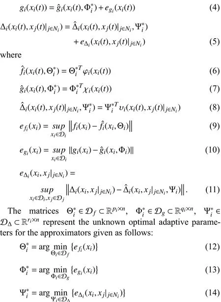
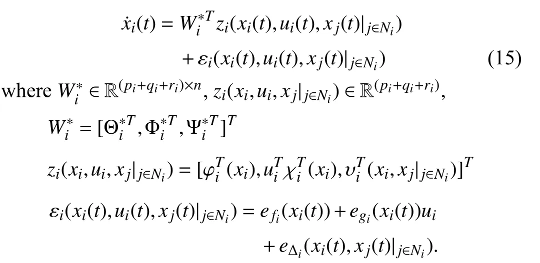
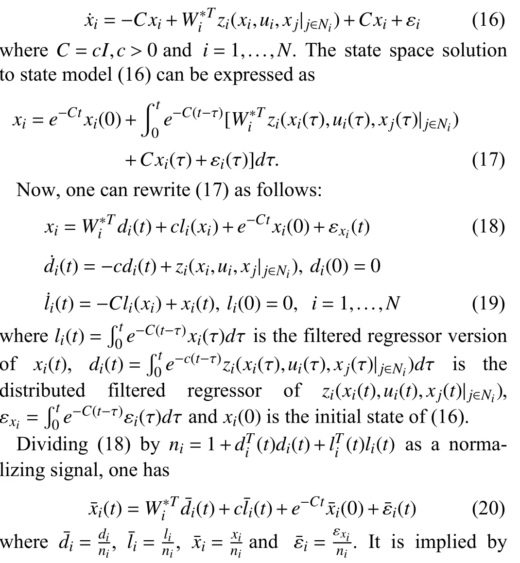
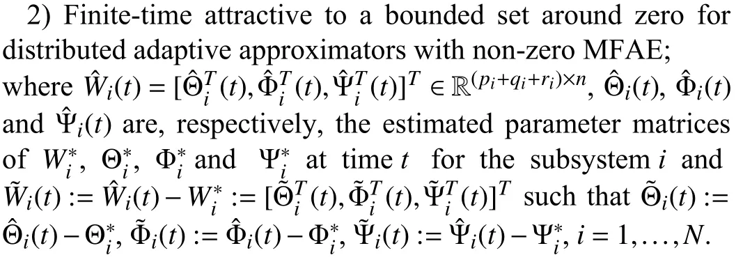
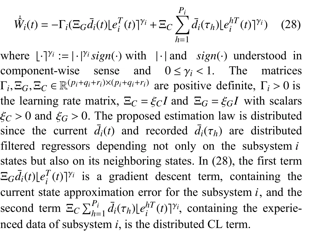
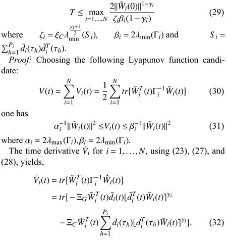
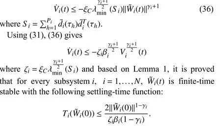
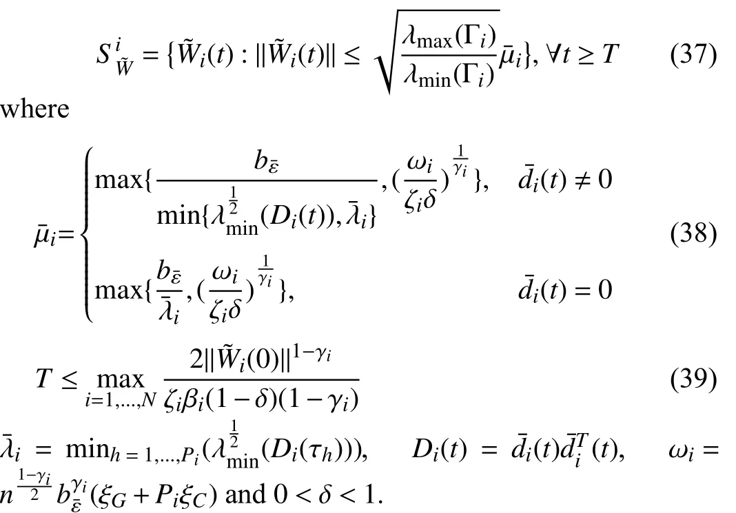
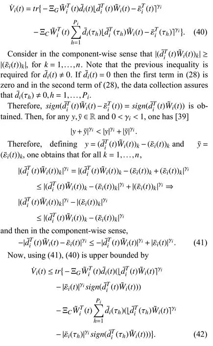
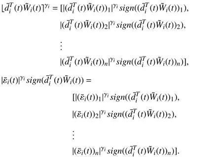
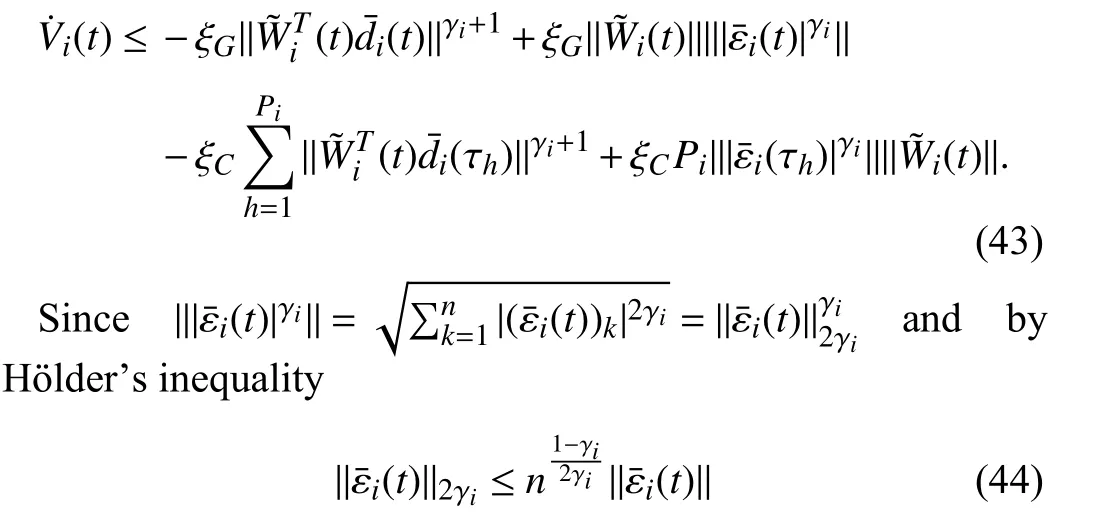
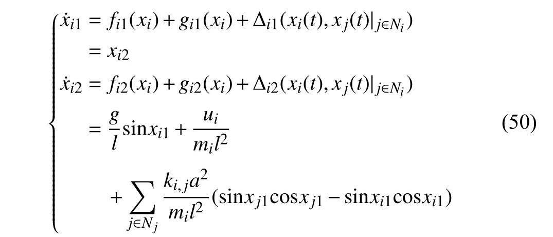
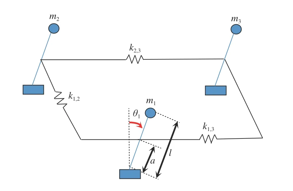
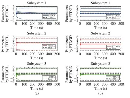
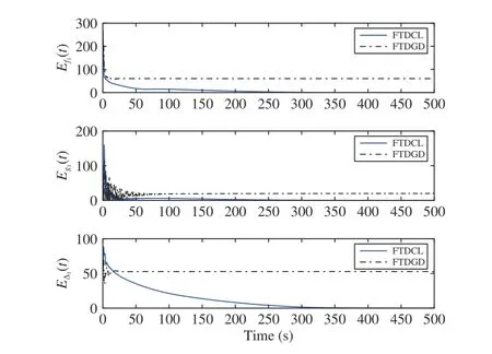
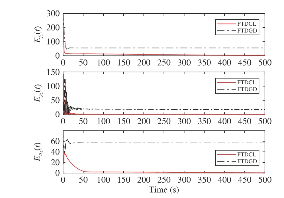
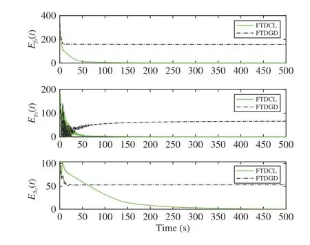
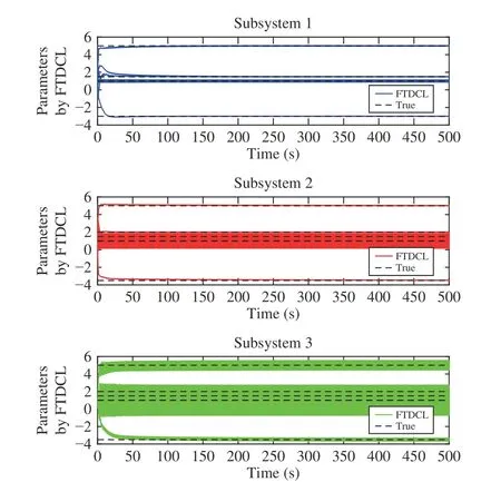
Lemma 1 [32]:Suppose that there exists a positive definite continuous functionV:DyR+∪{0} in an open neighborhood of the origin and there exist real numbers α>0 and 0 Then, the system (1) is finite-time stable with a finite settling-time for ally0∈Dy. Consider the following nonlinear interconnected system composed ofNuncertain subsystems described by: wherexi=[xi1,xi2,...,xin]∈Di⊂Rnis the state andui∈Du⊂Rmis the control input of subsystemi,i=1,...,N;Diand Duare compact sets.fi:DiRn,gi:DiRn×mand∆i:DNiRnare the unknown nonlinear drift, input and interconnection terms with DNi⊂Rn(|Ni|+1), respectively. This paper aims to present an identification method to learn the unknown dynamics of the nonlinear interconnected system(2) in finite time and in a distributed fashion.In order to learn the subsystems’ uncertain dynamics in a distributed fashion, first, every subsystem dynamics (2) is formulated into a distributed filtered regressor form. The distributed filtered-regressor form presents the subsystems’states with a time-varying regressor for which the dynamic flow of regressors are known and depend on the subsystem’s states and inputs, as well as its neighbors’ states. This will allow to present update laws without requiring to measure the state derivatives of the subsystems and their neighbors [13]. To develop filtered regressors, linearly parameterized adaptive approximation models are first used to respectively representfi(xi),gi(xi)and ∆i(xi,xj(t)|j∈Ni) for every subsystemi,i=1,...,Nas follows: and φi:DiRpi, χi:DiRqi, υi:DNiRriare the basis functions, such thatpi,qiandriare the number of linearly independent basis functions to approximatefi(xi),gi(xi) and∆(xi,xj|j∈Ni), respectively. The quantitiesefi(xi),egi(xi) ande∆i(xi,xj|j∈Ni), defined in (9)−(11) are, respectively, the MFAEs forfi(xi),gi(xi) and ∆i(xi,xj|j∈Ni), denoting the residual approximation errors for the case of optimal parameters. As a special case, if the adaptive approximation models(xi,Θi),(xi,Φi) and(xi,xj|j∈Ni,Ψi) can exactly approximate the unknown functionsfi(xi),gi(xi) and∆i(xi,xj|j∈Ni), respectively, then,efi=egi=e∆i=0. Remark 1:Generally, adaptive approximators can be classified into linearly parameterized and nonlinearly parameterized [13]. Linearly parameterized approximators are more common in the literature of adaptive control because they provide mechanism to derive stronger analytical results for stability and convergence. Linearly parameterized approximators are different and more general than linear models. In linear models, the entire structure of the system is assumed to be linear. In linearly parameterized approximators,the unknown nonlinearities are estimated by nonlinear approximators, where the weights (parameter estimates)appear linearly with respect to nonlinear basis functions. Remark 2:The linearly parameterized approximation models asgivenin (6)–(8), are linear inparameters,,and, respectively, and theircorresponding basis functions φi(xi(t)) , χi(xi(t)), and υi(xi(t),xj(t)|j∈Ni),respectively,contain somenonlinearfunctions. We considertwo differentcases[40]: 1) In the first case, the hypothesis class is assumed to be realizable. That is, the identification is realizable as there is a perfect hypothesis within the hypothesis class (i.e., basis functions and their corresponding optimum weights) that generates no error. 2) In the second case, the hypothesis class is assumed to be not realizable (all system parameters make some identification error). For the first case, the nonlinear basis functions completely capture the subsystem dynamics(i.e.,efi(xi(t)),egi(xi(t))e∆i(xi(t),xj(t)|j∈Ni,givenin (9)−(11),are zero)andonlyparametric uncertainty exists and therefore,the MFAE is zero. For the second case, the basis functions cannot fully capture the dynamics of the subsystems and mismatch error exists and therefore, the MFAE is nonzero for all hypotheses. By using (3)−(8), each subsystem dynamics (2) can be rewritten as Assumption 2:The approximation error εiare bounded inside compact sets Di, Duand DNi. That is,supxi∈Di,x j∈Dj,ui∈Du//εi(xi,ui,xj|j∈Ni)//≤bεwithbε≥0. The approximators’ basis functions are also bounded in the mentioned compact sets. A distributed filtered regressor is now formulated to circumvent the requirement of measuring(t), and is leveraged by the update law later. For regressor filtering, the dynamics (15) is rewritten as 1) Finite-time stable for distributed adaptive approximators with zero MFAE; In this section, a finite-time distributed parameter estimation law for approximating the uncertainties of the nonlinear interconnected system (2) is presented. The convergence analysis of the proposed method is presented based on the Lyapunov approach. Consider the distributed approximator for subsystemito be of the form The state estimation error of the subsystemiis obtained as The state estimation errorei(t), which is later employed in the proposed parameter update law, is accessible online,because(t) is computed online by the approximator (21) and(t)is the normalized measurable state of the system.However, for the sake of parameter convergence analysis,using (20) and (21),ei(t) in (22) is rewritten as To use CL, that employs experienced data along with current data in the update law of the distributed identifier parameters, the memory dataisrecorded inthememory stacksMi∈R(pi+qi)×Pi,Li∈Rn×PiandXi∈Rn×Piforeachinterconnected subsystemi,i=1,...,Nat times τ1,...,τPias wherePidenotes the number of data points recorded in each stack of subsystemi. The memory stackMicaptures the interactive data samples for which their richness depends on collective richness of the subsystem’s state itself as well as its neighbors. The number of data pointsPi, fori=1,...,N, is chosen such thatMiis full-row rank and contains as many linearly independent elements as the dimension of the distributed filtered regressordi(t) (i.e., the total number of linearly independent basis functions forfi(xi),gi(xi) and∆i(xi,xj|j∈Ni)), given in(18), thatis called asrank condition onMiand requiresPi≥pi+qi+ri,fori=1,...,N. In order for the matrixMito be full-row rank, one needs to collect at leastpi+qi+rinumber of data samples. Therefore,one can check the full-row rank condition on the data matrixMionline after recordingpi+qi+rinumber of data points in the memory stacks of the subsystemi. Whenever the full-row rank condition onMiis satisfied, i.e.,one can stop recording data samples in the corresponding subsystem’s memory stacks. The error(t) for thehth recorded data is defined as follows: where is the state estimation at time 0 ≤τh Remark 3:In the distributed approximator (21), the received neighboring states appear in the distributed filtered regressor(t), as given in (19). Therefore, the richness of the local neighboring data affects the richness and rank condition satisfaction of the distributed data stored in memoryMi. Now, the finite-time distributed estimation law for the unknown parameters in the interconnected subsystemiapproximator (21) is proposed as Remark 4:In (28), the weightsandare not necessarily equal and one of the two estimation terms can be prioritized over the other by choosing appropriate ξCand ξG,respectively. Generally, in (28) choosing high learning ratesΓior weights ξCcan increase the convergence rate. However, it may also lead to chattering in the estimated parameters. Once combined with the control design, this chattering can result in poor control performance or even instability. Remark 5:For every distributed identifier that uses (28), the s haredneighboringstates onthe learningtimelength,not only affectthe current value of the distributedregressor,,but are also influential on the richness of the distributed memory employed in the second term of (28). This entirely discriminates the current work from single system’s finite-time CLbased identification methods [28]−[31]. In the following, the convergence properties for distributed adaptive approximators with zero and nonzero MFAEs are investigated. The theorem below shows that using the proposed finitetime distributed concurrent learning method (28), for distributed adaptive approximators with zero MFAEs, i.e.,(t)=0 , the estimated parameters(t) converge to their optimal values in finite time. Theorem 1:Let the distributed approximator for every nonlinear interconnected subsystemiin (2), be given by (21),whose parameters are adjusted by the update law of (28) with 0 ≤γi<1and a distributed filtered regressor given by (19),fori=1,...,N. Let Assumptions 1 and 2 hold. Once the fullrow rank condition onMi,i=1,...,Nis satisfied, then for everyith adaptive distributed approximator with zero MFAE,i.e.,(t)=0 , the distributed parameter estimation law (28)ensures finite-time convergence of(t) to zero for all interconnected subsystems within the following settling-time function: One knows that and based on Fact 1 holds for 0<γi+1<2. Therefore, using (32)–(34), one obtains Therefore, Therefore, the whole interconnected system dynamics can be identified in finite time within the following settling time: Corollary 1:Let the assumptions and statements of Theorem 1 hold. Then, for adaptive distributed approximators with zero MFAEs, i.e.,(t)=0 , the state estimation errorei(t)for every subsystemi,i=1,...,N, is finite-time stable. Proof:The proof is a direct consequence of Theorem 1. ■ Remark 6:As shown in (29), the settling time function of the identifier depends on the minimum eigenvalue of the distributed memory matrix, λmin(Si). Therefore, to improve the convergence speed, an optimization over recorded data can be performed to replace old data with new ones as more data becomes available to maximize the minimum eigenvalue of the distributed memory matrix to reduce the convergence time. The following theorem gives the finite-time convergence properties for the distributed parameter estimation law (28) of distributed adaptive approximators with non-zero MFAEs,(t)≠0, in interconnected systems’ identification. Theorem 2:Let the distributed approximator for nonlinear interconnected subsystem (2) given by (21), whose parameters are adjusted by the update law of (28) with 0<γi<1 and a regressor given in (19). Consider that Assumptions 1 and 2 hold. Once the full-row rank condition onMifori=1,...,Nis met, then for adaptive distributed approximators with nonzero MFAEs, i.e.,(t)≠0, the proposed parameter estimation law (28) guarantees that for every subsystemi,i=1,...,N, the(t)is finite-time attractive by the following bounded set: Proof:Choose the same Lyapunov function (30) that satisfies (31). The time derivation ofViemploying (23), (27)and (28) gives, Recall that in ⎿·⏋γi, |·| a ndsign(·) are employed in the component-wise sense, i.e., Therefore, using (33), (34), //(t)//≤1 and (42), one obtains holds for all 0 <2γi<2, it is given that Therefore, In the following, (45) is rewritten as: where 0 <δ<1. Hence, From (31) and (46), it follows that: where and by comparison principle one obtains then using (31), the above inequality ensures that(t)satisfies for allt Therefore, for every subsystemi,i=1,...,N, the solutions of(t) are finite-time attractive to the bound in (48) where Therefore, all the solutions of,i=1,...,Nfor the interconnected system are finite-time attractive to the bound given in (37) in the following settling time: Corollary 2:Let the assumptions and statements of Theorem 2 hold. Then, for adaptive distributed approximators with non-zero MFAEs, i.e.,(t)≠0, the state estimation errorei(t) for every subsystem i,i=1,...,N, is finite-time attractive. Proof:The proof is a direct consequence of Theorem 2. ■ Remark 7:In Theorem 2, for γi=0, using (31) and (45) it can be shown that for every interconnected subsystemi,i=1,...,N, if ζi>ωi,(t) is finite-time stable and the interconnected system can be exactly identified with zero MFAE. Remark 8:As discussed in [41], the concurrent learning approach is based on the combination of a gradient descent algorithm with an auxiliary static feedback update law, which can be viewed as a type of σ-modification [13] and allows the requirement on persistence of excitation to be relaxed by keeping enough measurements in memory. Here, the same extension is applied to the proposed distributed finite-time concurrent learning in (28). Theoretical support of this claim is provided in Theorem 2 to show the finite-time attractiveness of the proposed parameter update law (28) in case of nonzero MFAEs. Remark 9:For distributed adaptive approximators with nonzero MFAEs, the richness of the distributed data stored inMiinfluences the finite settling time as well as the error bound.Accordingly,(t) converges to a narrower bound in faster time by maximizing λmin(Si) that minimizes the error bound and the settling time respectively given in (37) and (39).Therefore, after the rank condition satisfaction, optimization over recorded data can improve the convergence results for every subsystem where one can replace new distributed samples with old ones inMi,i=1,...,N, if λmin(Si) increases to result in a faster convergence to a lower error bound.Remark 10:Similar to the concurrent learning literature[18], [21]−[25], [27], [29] and most system identifiers for nonlinear systems, in this paper it is assumed that the subsystem states are measurable. Even though the subsystems’states are measurable, the finite-time identification of interconnected systems without the persistency of excitation requirement is challenging. Online finite-time identification of the interconnected system dynamics under output measurements assumption is a direction for future research. This requires coupled distributed identifier and observer design for every subsystem to be able to identify the subsystem dynamics and observe its states interactively in finite-time. Remark 11:In the proposed finite-time distributed concurrent learning estimation law (28), if the concurrent learning term regarding the past historical data is eliminated, the following finite-time distributed gradient descent estimation law that only depends on the current distributed data is obtained as: withKi>0. According to the analysis provided in the previous theorems, similar results are obtained for the estimation law (49) provided thatt) is persistently excited for every subsystemi. The finite-time distributed gradient descent law (49) is similar to the estimation law for a single system in Algorithm 1 of [42] where the short finite-time input to state stability of the mentioned learning law (ensuring stability in a finite and limited time interval) has been proven,provided that the regressor(t) is nullifying in finite time. Now, the proposed finite-time distributed CL method performance for a nonlinear interconnected system identification is examined in comparison with the finite-time distributed gradient descent estimation method given in (49).The considered nonlinear interconnected system contains 3 inverted interconnected pendulums as depicted in Fig. 1.Every inverted pendulumi[43], subject to control inputuiis described by Fig. 1. Interconnection network of the physically interconnected inverted pendulums. wherexi1=θi(rad) is the angular position andxi2=(rad/s)isthe angular velocity,forthe invertedpendulumi,i=1,2,3.The gravity accelerationgisg≈10m/s2,miis the massoftheith rod (mi=0.25kg,i=1,2,3),lis the length of each rod(l=2m),ais the distance from the pivot to the center of gravity of the rod (a=1m),ki,j(kg/s2) is the spring constant which interconnects subsystemito subsystemj,j∈Ni, withki,j=kj,iandk1,2=k1,3=1.5,k2,3=2. In this system, due to the physical limitations,xidomain is defined byDi=[Di1,Di2]TwhereDi1=[−6,6] andDi2=[−4,4] fori=1,2,3. The initial states and parameters are chosen from the interval [−2,2] and stabilizing controllersui=−0.06xifori=1,2,3are employed. Every interconnected subsystemidynamics in (50) is unknown. For every subsystemi,i=1,2,3, the proposed finite-time distributed concurrent learning identifier employs the following basis functions: While the regressor vectorzi(xi,ui,xj|j∈Ni) is exciting over some time period, it is not persistently exciting. The relaxed excitation condition without the PE requirement is achieved without injecting any exciting probing noise to the subsystems’ controllers. Therefore, the approximation of (50) for every subsystemiis as follows: where based on the system descriptions, the true parameters for the three interconnected subsystems are as follows: We set Γi=3I, ξG=1, ξC=0.1, γi=0.5 fori=1,2,3. We chose ξG>ξC, to prioritize current data to the recorded data in the proposed learning method (28) andPi=10 ,i=1,2,3,which are set to be greater than 6, the number of independent basis functions for every subsystem. To have a fair speed and the precision comparison of the mentioned methods for approximating(xi) and(xi) on the domainDi, and(xi,xj|j∈Ni) on the domain ofDNi, the following online learning errors are computed for every subsystemi,i=1,2,3: Fig. 2. (a) Parameters of finite-time distributed concurrent learning(FTDCL) identifiers for subsystems 1–3; (b) Parameters of finite-time distributed gradient descent (FTDGD) identifiers for subsystems 1–3. Fig. 3. Online learning errors Ef1(t), Eg1(t) , and E∆1(t) for interconnected subsystem 1. Fig. 4. Online learning errors Ef2(t), Eg2(t) , and E∆2(t) for interconnected subsystem 2. Fig. 5. Online learning errors Ef3(t), Eg3(t) , and E∆3(t) for interconnected subsystem 3. It should be noted that Γi, ξGand ξC,i=1,2,3, are appropriately selected to adjust the learning speed and avoid chattering in the estimated parameters. In Fig. 6, it is shown that setting higher values for Γiand ξC( Γi=5I,i=1,2,3, and ξC=0.3) results in faster convergence of the estimated parameters; however, it also results in the undesired chattering of the estimated parameters. Fig. 6. Subsystems 1–3 unknown parameters’ estimation using inappropriate design parameters for finite-time distributed concurrent learning(FTDCL) identifiers. In this paper, a finite-time distributed concurrent learning method for interconnected systems’ identification in finite time is introduced. Leveraging local state communication among interconnected subsystems’ identifiers enabled them to identify every subsystem’s own dynamics as well as its interconnections’ dynamics. In this method, distributed concurrent learning relaxed the regressors’ persistence of excitation(PE) conditions to rank conditions on the recorded distributed data in the memory stack of the subsystems. It is shown that the precision and convergence speed of the proposed finitetime distributed learning method depends on the spectral properties of the distributed recorded data. Simulation results show that the proposed finite-time distributed concurrent learning has outperformed the finite-time distributed gradient descent in both terms of precision and convergence speed. For future work, we aim to develop finite-time distributed identifiers and observers to be employed in appropriate distributed controllers for interconnected systems.


B. Problem Formulation




III. FINITE-TIME DISTRIBUTED CONCURRENT LEARNING


A. Finite-Time Distributed Concurrent Learning Estimation Law
B. Finite-Time Convergence Properties for Distributed Adaptive Approximators With Zero MFAEs ((t)=0)



C. Finite-Time Convergence Properties for Distributed Adaptive Approximators With Non-Zero MFAEs ( (t)≠0)


IV. SIMULATION RESULTS


V. CONCLUSION AND FUTURE WORK
杂志排行
IEEE/CAA Journal of Automatica Sinica的其它文章
- An Overview and Experimental Study of Learning-Based Optimization Algorithms for the Vehicle Routing Problem
- Towards Long Lifetime Battery: AI-Based Manufacturing and Management
- Disagreement and Antagonism in Signed Networks: A Survey
- SwinFusion: Cross-domain Long-range Learning for General Image Fusion via Swin Transformer
- Real-Time Iterative Compensation Framework for Precision Mechatronic Motion Control Systems
- Meta Ordinal Regression Forest for Medical Image Classification With Ordinal Labels
