Property estimation of free-field sand in 1-g shaking table tests

Xu Chengshun, Jiang Zhiwei , Du Xiuli, Deng Lijun and Li Zheng

1.College of Architecture and Civil Engineering, Beijing University of Technology, Beijing 100124, China

2.National Engineering Research Center of Green & Safe Construction Technology in Urban Rail Transit, Beijing Urban Construction Design and Development Group Co., Ltd., Beijing 100037, China

3.Department of Civil Engineering, Tsinghua University, Beijing 100084, China

4.Department of Civil and Environmental Engineering, University of Alberta, Edmonton T6G2R3, Canada

5.Université Gustave Eiffel, Département GERS, Laboratoire Centrifugeuses Géotechniques (CG), Bouguenais 44341, France

Abstract: Experimental data taken from free-field soil in 1-g shaking table tests are valuable for seismic studies on soilstructure interaction.But the available data from medium- to large-scale shaking table tests were not abundant enough to cover a large variety of types and conditions of the soil.In the study, 1-g shaking table tests of a 3-m-height sand column were conducted to provide seismic experimental data about sand.The sand was directly collected in-situ, with the largest grain diameter being 2 cm and containing a water content of 6.3%.Properties of the sand were estimated under the influence of white noise plus pulse and earthquake motions, including the settlement, the dynamic properties of the sand column, and the three soil layers′ shear modulus degradation relationships.The estimated properties were then indirectly verified by means of finite element analysis.Results show that the estimated parameters were effective and could be used in numerical modeling to reproduce approximate seismic responses of the sand column.

Keywords: 1-g shaking table test; seismic sand response; dynamic soil properties; free-field sand

1 Introduction

The 1-g shaking table test is a valuable experimental method for seismic studies of soil-structure interaction,such as studies on subway stations (Kheradiet al.,2018), tunnels (Jianget al., 2010; Yuet al., 2018; Xuet al., 2021, 2022), and piles (Gerolymoset al., 2010;Cengiz and Guler, 2018).Because the seismic response of structures will be notably influenced by the seismic response of free-field soil, the seismic behavior of freefield soil is often desired prior to the testing of complex soil-structure systems on a shaking table.For example,Chenet al.(2010) performed 1-g shaking table tests of free-field soil as a step prior to conducting tests on utility tunnels.Yanet al.(2015) carried out multi-point shaking table tests of the free field to shed light on the dynamic soil-tunnel response.Moghadam and Baziar (2016)conducted free-field tests to ascertain the performance of the absorbing boundary of a box before performing 1-g shaking table tests on subway stations.

These studies show that the free-field tests were meaningful preliminary studies on soil-structure interaction.The experimental data or identified soil properties (Sadrekarimi, 2013; Tsaiet al., 2016; Dihoruet al., 2016) arrived through free-field tests were helpful for subsequent experimental designs or complementary numerical analyses.However, although 1-g shaking table tests on free-field sand have widely been conducted,and a large amount of experimental data were provided(Fishmanet al., 1995; Anastasopouloset al., 2008; Liet al., 2015; Lombardiet al., 2015), the available data from medium- to large-scale shaking table tests were not sufficiently abundant to cover a large variety of types and conditions of the soil.Experimental data regarding free-field soil are still needed for the design of 1-g shaking table tests, as well as numerical simulations on soil-structure interaction.

In the study, 1-g shaking table tests (STT) of a 3-m-height sand column were carried out.The sand was directly collected from a site at a depth of 20 m in Beijing, with a largest grain diameter of 2 cm and a water content (w) of 6.3%.The objective of the studywas to provide experimental data and properties of the sand column through STT, including the dynamic properties of the sand column, as well as three-layer shear modulus degradation and damping relationships,etc.The characterized properties were then indirectly verified using finite element modeling.

2 Experimental programs

A series of shaking table tests of a sand column were carried out in the present study.The following subsections describe the geotechnical properties of the soil, the experimental setup, instrumentation, and input motions.

2.1 Properties of sand

The sand was collected at an underground construction site in Beijing, China.Figure 1 shows grain size distribution and the physical properties of the sand in the shaking table test.The values of the coefficient of uniformity (Cu), coefficient of curvature (Cc) and median grain diameter (D50) were 8.3, 0.75 and 0.82 mm,respectively.With a fines content of less than 2%, the soil was classified as poorly-graded sand (SP) according to the Unified Soil Classification System.The initial total unit weight (γt) of the soil built in the shaking table container was 17.6 kN/m3.The values of the maximum and minimum void ratio (emaxandemin) were 0.92 and 0.43, respectively.

2.2 Equipment and model soil construction

The STT was conducted at the China Academy of Building Research, Beijing, China.The operating frequency of the shaking table equipment was in the range of 0.1 Hz to 50 Hz.

Because the laminar shear box could have flexible shear deformation responses at the boundary and could be used to mimic a 1-D seismic deformation of the soil,the laminar shear box was applied in the tests.The size of the soil container was 3.2 m × 2.4 m × 3 m (length ×width × height) and a 1-cm-thick rubber membrane was arranged along the inner walls of the box.The laminar rings were unconstrained in the direction of length but constrained by steel braces in the direction of width.Figure 2(a) shows the shaking table and the laminar shear box.Each frame comprising the box had a height of 12 cm, and the frames were supported with rollers.The predominant frequency of the empty box (without soil) was 0.83 Hz, while the predominant frequency of the full box (with soil) was in the range of 6.39 Hz to 9.08 Hz(and will be introduced in subsequent sections).The box and soil could hardly have resonance responses.It is suggested that seismic responses of the box could not notably influence seismic responses of the soil.

The sand was manually filled and carefully compactedabout every 10 cm lift until the box was full.Sensors were buried at designated locations in the soil during processes of filling and compaction.Input base motions were excited at the bottom of the box lengthwise.

2.3 Instrumentation

A total of 35 accelerometers, three laser displacement sensors (LDS) and a Shape Acceleration Array (SAA)were used in the tests.Figure 2(b) shows the arrangement of the sensors.

The acceleration was recorded using built-in IC(integrated circuit) accelerometers.The sensitivity,frequency range -3dB and noise density of accelerometers were 300 mV/V, DC-2500 Hz and 0.15 mg/rt-Hz,respectively.The accelerometers were named Channeln, i.e., CHn(n=01, 02, …, 35).CH01 was placed on the shaking table to record input motions imposed by the shaker.CH02-CH29 were buried in the box to record the soil response, and CH30-CH35 were used to record motions of the box.The sampling frequency of the accelerometers was 256 Hz.

The LDS were hung above the ground surface to record the settlement of sand.The resolution, effective measurement range and sampling frequency of LDS were 13 μm 200 mm and 5 Hz, respectively.

The SAA was a flexible plastic tube that had a Microelectro Mechanical System (MEMS) embedded in it.The SAA was buried in the soil so that it could record its deformation.It had been proved effective to monitor the lateral deformation of the soil, both in the field (Abdounet al., 2013) or via experiments done in a laboratory(Linet al., 2015), as noted in the literature review.In the present tests, the SAA was used to measure the lateral deformation under the influence of the static condition.Figure 2(b) shows the arrangement of the SAA.The diameter of the SAA tube was about 32 mm and the accuracy of the recorded deformation was about 0.1 mm.

2.4 Input motions

A white noise, a pulse motion and four earthquake motions were selected as input motions for the STT.Figures 3(a) and 3(b) show the time histories of the white noise and pulse motions recorded at the base.The white noise motion was used to determine the predominant frequencies of the sand column.The pulse motion was used to create a shear wave transmitting through the soil to obtain the shear wave velocity of the soil.It also was used to determine the small-strain damping ratio according to the free-vibration of the soil.In sum, the white noise and pulse motions were each input five times during the STT.

The input earthquake motions included three natural motions and one artificial motion.The natural motions were selected from the Loma Prieta earthquake(Gilroy Array #3 station H20F*, USA, 1989), the Kobe earthquake (KJMA station H1*, Japan, 1995) and the Sichuan earthquake (20-40 s, 51WCW station EW,China, 2008).(*Downloaded from the PEER Ground Motion Database, Pacific Earthquake Engineering Center: https://ngawest2.berkeley.edu).As the soil was collected at Beijing, the artificial motion was created according to native site design parameters and spectra(GB 50011, 2010; GB 18306-2015, 2015).

The predominant frequencies of motions were scaled for the STT in an attempt to saddle the estimated predominant frequency of the sand specimen to obtain the strongest responses.However, as the laminar box was unconstrained in the shaking direction, the responses of the soil and box were limited to ensure the safety of the equipment and personnel.The scaling factors (prototype/model) for frequencies of the Loma Prieta earthquake(LP), the Kobe earthquake, the Sichuan earthquake (SC)and the Beijing artificial earthquake (BJ) were finally taken as 1/3, 1/4, 1/3 and 1/2, respectively.However,since the actual predominant frequency of the sand specimen was notably changed by the input sequence,predominant frequencies of scaled input motions were not consistent with predominant frequencies of the sand specimen during the course of the test.

Table 1 shows the sequence of input motions (IM),which were divided into four stages, i.e., the 0.2 g, 0.4 g,0.62 g and 1.0 g stages, differentiated by the peak acceleration (apk) of input motions.Figure 4 shows the input seismic motions recorded on the surface of the shaking table and their peak Fourier amplitude at the 0.2 g stage.The frequency content of base motions were similar in the subsequentapkstages and only a slight discrepancy ofapkwas observed due to the performance of the shaking table equipment.

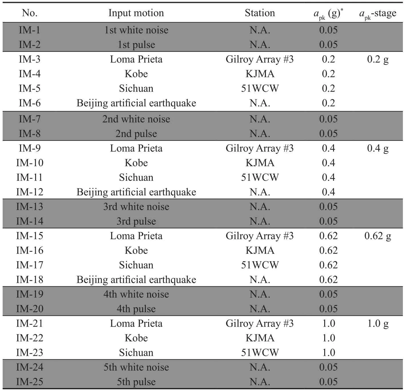
Table 1 Input motion sequence

Fig.3 Input dynamic motions: (a) white noise and (b) pulse motion

The white noise and pulse motions were both input at the beginning and at the end of each stage, with a smallapkof 0.05 g.After a motion was exerted, waiting time was employed to observe the experimental phenomena.Because large residual displacements of several laminar rings at the top of the box were considerably large (about 0.2 m) at the end of IM-23, seismic input was terminated after IM-23 due to safety concerns.

3 Tests results

In this section, typical results of the shaking table tests are presented and discussed.The properties of the sand were estimated using results of white noise, pulse,and earthquake motions.

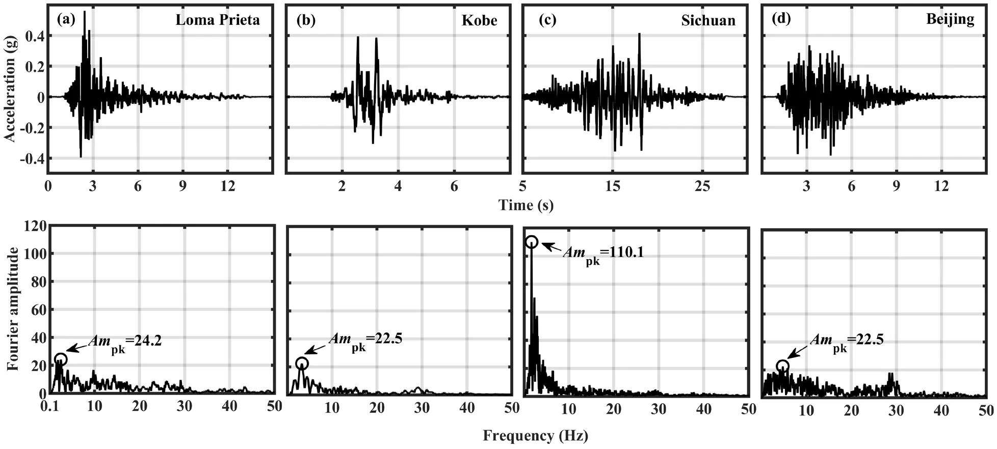
Fig.4 Input seismic accelerations and their Fourier amplitude, with peak amplitude (Ampk): (a) Loma Prieta, (b) Kobe, (c) Sichuan and (d) Beijing.These motions are at the 0.2 g stage, recorded at the shaking table

3.1 Typical experimental data and observation

Because dynamic soil properties will be backcalculated using time-histories of acceleration, the results owing to the Loma Prieta motion were selected for presentation due to the limited length of this paper.Figures 5 and 6 show acceleration results at the 0.2 g,0.4 g, 0.62 g and 1.0 g stages.Estimation of dynamic soil properties will be introduced in subsequent sections.

The SAA could follow the deformation of the soil,and the accumulated lateral soil deformation could be directly measured using the SAA.The results of residual displacement could serve as a supplement for the integral displacement, because residual displacement could not be preserved due to the filtering effect in calculating the displacement by using time-integration of acceleration records.Figure 7 shows the accumulated lateral shear deformation of the soil recorded by the SAA.

The values of lateral displacement at the soil surface during theapkstages were 0.67 mm (at IM-7), 1.87 mm(at IM-13), 11.0 mm (at IM-19) and 106.2 mm (at IM-24), respectively.The lateral deformation of the soil was accumulated withapkstages, especially for the soil at the elevation ranging from 2 m to 3 m whenapkwas greater than 0.62 g.The lateral residual displacement of the soil at anapkstage did not follow a regular deformation pattern along the elevation, which might be due to the complex loading history of the seismic motions.

Figure 8 shows the final state of the soil and box.As the vertical settlement at the soil surface reached 103.35 mm, the movement of the top ring could hardly be constrained by the soil.The large residual displacement(LRD) of the laminar rings was observed at the top of the soil toward the end of the tests.The value of LRD was about 20 cm at IM-23.To prevent the fall of the ring,seismic tests were terminated, for safety concerns.

3.2 Validity of shear deformation mode

The laminar box was used to mimic the onedimensional (1-D) condition for the soil.A 1-D soil column would have the shear deformation mode under seismic actions, and therefore displacements at different positions of an elevation would have approximately identical values during the shaking.For the present tests, values of peak displacement at elevations were compared to validate the shear deformation mode of the sand column.The displacement was acquired via double-integration for time-histories of acceleration and hereafter.The cumulative trapezoidal numerical integration method was used to execute doubleintegration.During the integration processes, a band-pass zero-phase digital filter was used to conduct filtering in a frequency range from 0.5 Hz to 40 Hz.The 0.5-40 Hz band pass filtering was proved effective to deal with the zero drift and high-frequency noise of the acceleration signal (Liet al., 2013).

Table 2 shows values of peak displacement at three elevations under the Sichuan motion.Discrepancies among values of peak displacement at three elevations were very slight during the fourapkstages.The largest relative difference was observed at the top of thesoil (i.e., CH15 and CH29) at the 1.0 g stage, but the value was only about 5%.This implied that the soil in the box followed shear deformation during the tests.The boundary effect of the container had a very slight influence on the dynamic responses of the soil.The test results were good for performing subsequent analyses.

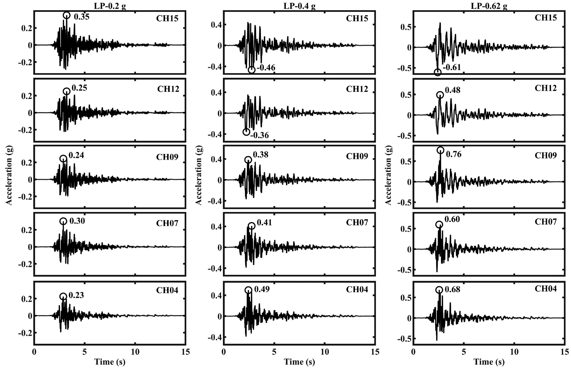
Fig.5 Time histories of acceleration under Loma Prieta motion at 0.2 g, 0.4 g and 0.62 g stages

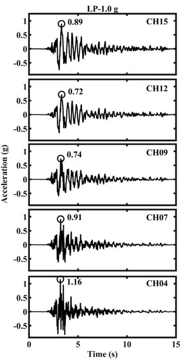
Fig.6 Time histories of acceleration under Loma Prieta motion at the 1.0 g stage

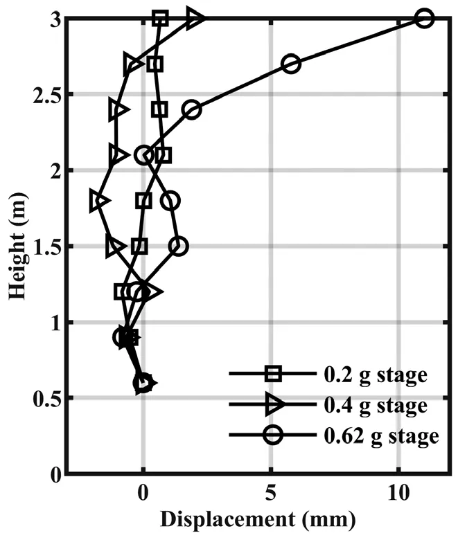
Fig.7 Accumulated lateral shear deformation of soil at depths from 0 to 2.4 m

3.3 Dynamic properties of the soil column

As the white noise was a wide band excitation, the sand column would develop resonance at predominant frequencies.Figure 9(a) shows transfer functions under white noises at CH15 and CH07.The transfer functions in the figure were smoothed, with a smoothing length of 40.The 1st and 2nd mode frequencies (f1andf2) were about 9.08 Hz and 28.78 Hz at IM-1, according to peaks of transfer functions and their phase angles (Liet al.,2013).The same method was used to obtain predominant frequencies at subsequent white noise motions and values off1andf2, as summarized in Table 3.The values off1andf2significantly decreased at the 0.2 g and 0.4 g stages, but they were almost steady after the 0.4 g stage,even if great settlement and lateral displacement were observed in the 0.62 g and 1.0 g stages (Fig.8).

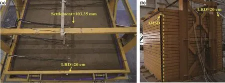
Fig.8 Final state of soil and box: (a) top view; (b) overview.ALSD means accumulated lateral shear deformation, and LRD is large residual displacement

The damping ratios could be obtained by using responses under pulse motions.After a pulse motion was loaded, the response of the deposit was damped off under the free vibration.Figure 9(b) shows the acceleration response of CH15 due to IM-2.The logarithm decrement method (Chopra, 2007) was used to calculate the viscous damping ratio (ξ) of the soil when subjected to pulse motions.As observed in Table 3,ξincreased withapkpossibly because the deposit experienced a greater shear strain.

3.4 Properties variation due to settlement

Settlement of the sand was observed during the course of the shaking.Table 4 shows the average accumulated settlement as recorded by laser sensors (LA01, LA02 and LA03 in Fig.2(b)).Because of settlement, the volume of the soil decreased at eachapkstage.γtwas also various and ranged from 17.6 kN/m3to 18.2 kN/m3at differentapkstages.The soil was densified due to changes in the volume andγtof the soil.The corresponding average relative density (Dr) of the soil varied from 68.6% to 78.9%.The values ofecould then be obtained due to the change inDr.Both values ofγtandDrgradually increased during the tests.Table 4 summarizes the values of accumulated average settlement,γt,Drandeatapkstages.

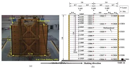
Fig.2 Test setup: (a) shaking table and laminar box; and (b) schematic diagram of the sensor arrangement

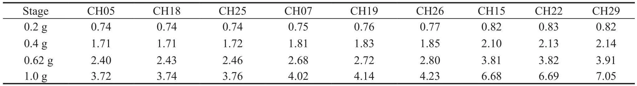
Table 2 Comparison of peak horizontal displacement at three elevations under Sichuan motions (unit: cm)

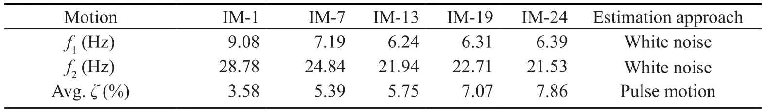
Table 3 Frequencies and average damping ratio of the soil column

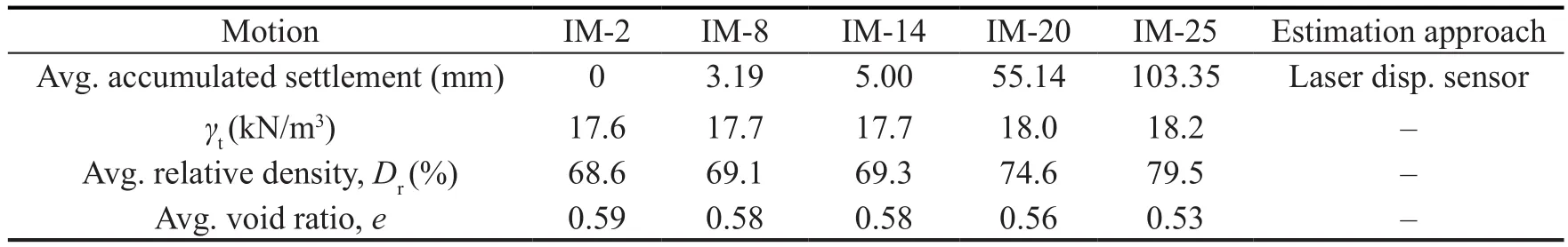
Table 4 Properties of soil measured among stages

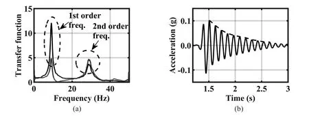
Fig.9 Responses of soil under white noise and pulse motions: (a) transfer functions under white noise at IM-1; (b) time-history of acceleration at CH15, IM-2

3.5 Estimation of Gmax

When a pulse motion was excited, a shear wave was transmitted from the bottom to the top of the soil.The average transition time could be attained by counting the time lag of the first peak from CH01 to CH15.Figure 10 shows the time lag of pulses.The average shear wave velocity (Vsp) of the soil could then be computed byhs/t,wherehsis the height of the soil column andtis the time lag between first peaks of CH01 and CH15.Table 5 shows the values ofVsp.

The average shear wave velocity of the soil can also be estimated via:

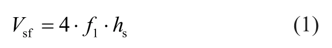
whereVsfis the average shear wave velocity, estimated using the predominant frequencies.Table 5 summarizes the values ofVsf.There was a slight discrepancy between the estimatedVsfandVsp.This might be due to the slight nonlinearity of the soil, caused by the white noise and pulse motions.

The values of shear wave velocity (Vs) at elevations should have been well calculated by counting the time lags of the soil under pulse motions, using a highperformance data acquisition system in centrifuge tests(Brennanet al., 2005; Liet al., 2013).However, the sampling frequency of accelerometers in the 1-g shaking table tests was usually much lower than those for the centrifuge tests.Therefore, the values ofGmaxwere often estimated using back-analysis or empirical methods.Tsaiet al.(2016) estimatedGmaxby matching the shear modulus reduction results obtained from STT with curves derived by Seed and Idriss (1970).Dihoruet al.(2016) estimatedGmaxusing aliasing frequencies and a critical shear wavelength.Sadrekarimi (2013) and Anjaliet al.(2015) calculatedGmaxvia empirical equations and parameters.

In the present tests, values ofVswere estimated in three layers via the back-analysis method.When conducting back-analysis,Vsof a sand layer was estimated and checked by considering the following criteria: (1)fitting the time-lag of pulses along the elevation to acquire values ofVsin three layers.An average shear wave velocity (VsG) of the 3-m-height sand column could be acquired using the fittedVs.The values ofVsGwere then checked by comparing them with values ofVspandVsf.(2) referencing the shear modulus degradation relationships (γ-G/Gmax) from published literature; (3)applying the estimated maximum shear modulus (Gmax),taken from finite element modeling of the sand column,which will be introduced in a subsequent section.

Figure 10 shows fitted time lags of pulse motions in three sand layers.The thicknesses of Layer 1 (L1), Layer 2 (L2) and Layer 3 (L3) from the top to the bottom of the soil were 0.79 m 1.04 m and 1.1 m, respectively.For the initial condition, there might be a discrepancy when conducting the fitting at IM-2.This task was limited by the sampling frequency of accelerometers, which could hardly capture a very short time transmission due to a larger soil shear modulus.In the laterapkstages,predominant frequencies of the sand column were decreased, and time lags were long enough to effect the fitting.The values ofVsGwere acquired via the fittedVsin three layers duringapkstages.They were checked by comparing them with the values ofVspandVsf.Table 5 shows the values ofVsG,VspandVsf.Although there were slight differences among them, they matched fairly well.The values ofVsGwere good.This suggests that the estimated values of theVsfor the three sand layers were also reasonable.

The average shear moduli of the three layers (G1,G2andG3) could then be computed using values ofVsandγtatapkstages.Table 5 shows the values ofG1,G2andG3.As they were estimated at the beginning ofapkstages,G1,G2andG3were the maximum shear moduli for dynamic soil properties atapkstages.

Table 5 Estimated shear moduli (unit: MPa) and shear wave velocities (unit: m/s) of sand

3.6 Estimation of γ-G/Gmax

This section introduces the estimation of shear modulus degradation vs.shear strain by using dynamic records under the influence of earthquake motions.The time histories of shear strain at CHi(i=2, 3, …, 14) can be estimated using Eq.(2) (Zeghalet al., 1995; Liet al.,2013) under earthquake motions:

whereγiis the time-history of shear strain at the CHielevation;uiis the time-history of displacement at theCHielevation; andhis the distance between CHi+1 and CHi, as shown in Fig.2(b).

The shear stress at an elevation can be estimated by using Eq.(3) (Zeghalet al., 1995; Liet al., 2013):

whereτiis the shear stress at the CHielevation;u˙iis the acceleration at the CHielevation;ziis the distance from the soil surface to CHi; andρis the soil density.Then the shear stress-shear strain hysteresis of the soil at an elevation could be obtained by utilizing Eqs.(2)and (3).

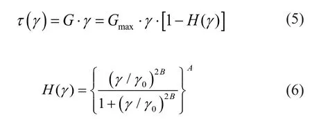
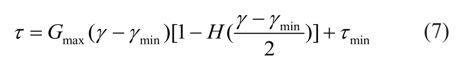
Figure 11(a) shows the typical shear stress-shear strain hysteresis, measured at CH04, CH08 and CH13 of IM-11.The shear strain, depending on the shear modulus(G) of the sand, could be calculated from each hysteresis loop, as introduced by Zeghalet al.(1995), Brennanet al.(2005) and Liet al.(2013).At the 0.4 g stage, the values ofGunder the four earthquake motions could be acquired using the method depicted in Fig.11(b).The values were then normalized usingGmaxobtained at initials ofapkstages, i.e.,G1,G2andG3, as summarized in Table 5.Figure 12 shows the normalized shear modulus degradation relationships at CH13, CH08 and CH04 (0.4 g stage).The shear modulus degradation relationships at other stages could also be obtained using the same method.

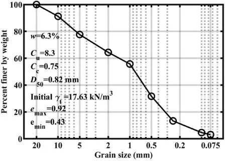
Fig.1 Physical properties and grain size distribution of sand in the shaking table test

Fig.11 Shear stress-strain loops at IM-11 and the method for calculating dynamic soil properties: (a) hysteresis derived from records at CH04, CH08 and CH13; (b) schematic of methods for estimating the shear modulus and damping ratio

The degraded shear modulus data obtained from hysteresis loops were slightly scattered, as demonstrated in Fig.12.This might be becauseVs,γtandeof the soil were variables during shakings.Variations of properties were included in estimations.Additionally, the rotation or displacement of the buried accelerometers could also influence the estimation.Such scattering phenomena were also reported by Zeghalet al.(1995), Brennanet al.(2005), and Rayhani and Naggar (2008).

Because the model proposed by Darendeli (2001)and Menq (2003) (D & M model) has been widely used in seismic site analysis (Hashashet al., 2017), theγ-G/Gmaxrelationship calculated from the D & M model was compared with dynamic soil properties estimated from the present tests.

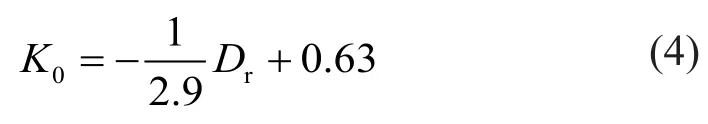
According to the D & M model, the lower and upper limits ofγ-G/Gmaxcould be computed according to values of the confining pressure (σ′o), a 0.014% standard deviation of the reference strain, and a 0.09 standard deviation of the curvature coefficient (Menq, 2003).The value ofσ′oat CH08 could be estimated using the lateral earth pressure coefficientK0, and vertical effective stress,σ′v.K0, can be expressed by Eq.(4) (Gaudin, 1999):

Asσ′vwas about 24.2 kPa at the CH08 elevation, andσ′o=14.3 kPa was applied to the D & M model.Figure 12 shows the range ofγ-G/Gmax, obtained from the D& M model.As depicted in Fig.12,γ-G/Gmaxfrom the STT and D & M models matched well, which suggests that the values ofGmaxandGwere properly estimated.

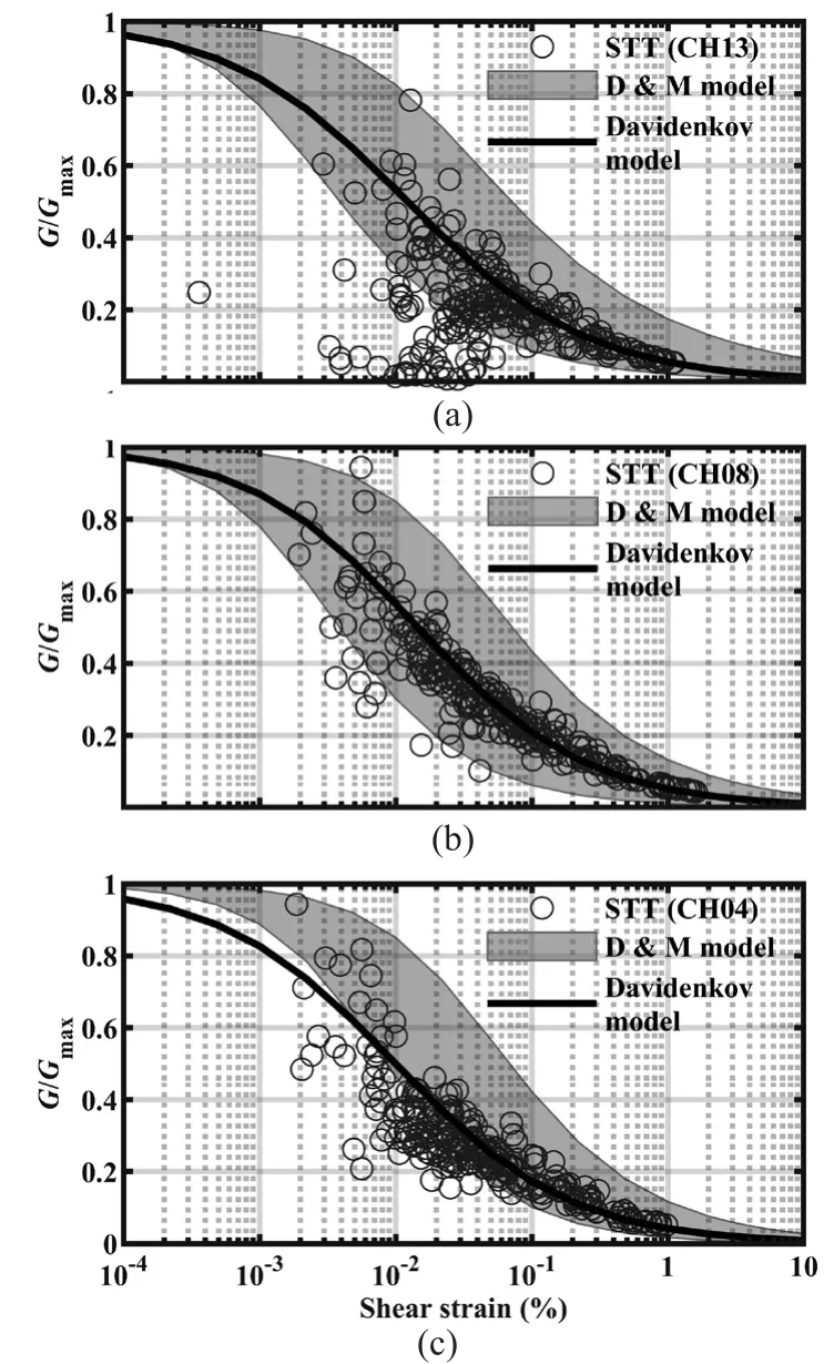
Fig.12 Shear modulus degradation obtained from the shaking table test (STT, 0.4 g stage), D & Q model (Darendeli,2001; Menq, 2003), and the fitted Davidenkov (Martin,1975) model used in FEM: (a) at CH13; (b) at CH08 and (c) CH04

3.7 Properties described using Davidenkov model

The Davidenkov model (Martin, 1975) was proved highly efficient and effective in numerical analyses for the seismic site response and soil-structure interactions(Martin and Seed, 1982; Chenet al., 2015a; Chenet al., 2015b), and therefore was selected for performing the finite element analysis of the sand column.The soil properties described using Davidenkov model would be applied to the numerical modeling, which will be introduced in the subsequent section.

The Davidenkov constitutive model is a non-linear viscoelastic hyperbolic model for assessing soil dynamic behavior.The backbone curve of the model can beexpressed as:

whereHis a function ofγ;AandBare fitting coefficients andγ0is the reference strain (Hardin and Drnevich, 1972).

Figure 11(b) shows the stress-strain loops of the Davidenkov model.The loops were constituted using the Masing rules (Martin and Seed, 1978), composed of uploading and unloading sections, which can be described as Eqs.(7) and (8), respectively:

uploading:

unloading:

whereτminandτmaxare the minimum and maximum stresses, respectively, as shown in Fig.11(b).The damping ratio of the Davidenkov model was then identified through strain-dependent loops, using values ofWsandWDas shown in Fig.11(b), whereinWsis the area of the shaded triangle andWDis the area of the loop.

Parameters were attained by fitting theγ-G/Gmaxdata estimated in four stages, respectively.Figures 12(a), 12(b)and 12(c) show fitted curves using the Davidenkov model at CH13, CH08, CH04 (0.4 g stage), respectively.Table 6 summarizes the fitted parameters of the Davidenkov model.The parameters of the Davidenkov model at the 0.2 g, 0.4 g, 0.62 g and 1.0 g stages were named S2, S4, S6 and S10, respectively.Rayleigh damping was also incorporated in the numerical simulations to supply small strain damping.Coefficientsαandβwere computed usingf1,f2andξfrom Table 3, via Eq.(9),introduced by Chopra (2007).

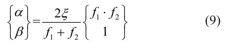
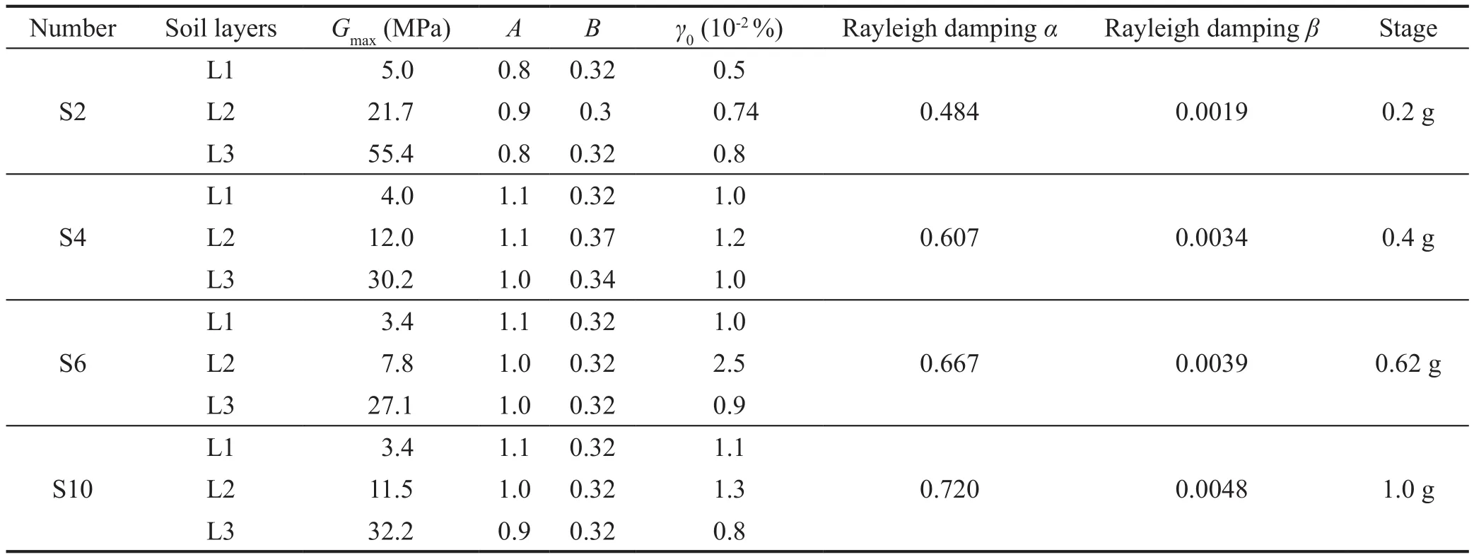
Table 6 Fitted parameters of the Davidenkov model

4 Parameters indirectly verified using numerical modeling

The finite element modeling of the 3-m-high sand column was conducted to indirectly verify the effectiveness of estimated parameters.The modeling was performed using finite element software ABAQUS.

4.1 Numerical model

A simple 3-D finite element model of the soil column was used to study responses in tests because a 3-D model would have a broader application on seismic studies of soil-structure interaction.Figure 13 shows the finite element model of the soil.The size of the numerical model was identical to that of the soil in the STT.The soil was divided into three layers along the elevation as the division point when estimating the values ofVs, as depicted in Fig.10.The computational thicknesses of three soil layers were 0.86 m (Layer 1), 1.04 m (Layer 2) and 1.10 m (Layer 3), respectively.The Davidenkov model was compiled as a VUMAT user subroutine for ABAQUS.The parameters in Table 6 were applied for the material properties of the soil layers.Nodes on the boundaries along the shaking direction of the soil were tied together to simulate the constraint provided by laminar rings used in tests.A similar simplified boundary condition was proved effective, and the reflection of seismic waves had a slight influence on the modeling results (Tsinidiset al., 2016).Zero displacement boundary conditions along the width and height of the soil (i.e.UzandUy) were applied to the numerical model.The accelerations recorded on the shaking table were excited along the length at the bottom of the model.Before acceleration was loaded, 1-g initial geo-stress was applied.

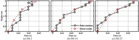
Fig.10 Time lag under pulse motions and their fitted results: (a) IM-2; (b) IM-14; (c) IM-25

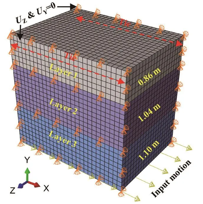
Fig.13 Finite element model of soil

4.2 Numerical results

The numerical results of displacement were compared with test results at the 0.2 g, 0.4 g and 0.62 g stages.Figures 14 and 15 show the numerical results of the displacement and their Fourier spectra computed by using parameters of S2 and S4, respectively.The time-histories and spectra of the displacement matched very well with test results for all three soil layers.But in the later stage, the divergencies were larger (Figs.16 and 17).This might be because accelerometers were vertically displaced due to the large settlement of soil from the 0.62 g stage, and the buried accelerometers might possibly have had rotation responses under strong motions in tests, while the settlement and rotation effects were not incorporated into the modeling.This was the case even though parameters were still accepted, because the discrepancy between numerical and test results was slight.

The numerical results suggest that seismic responses of the sand column in shaking table tests were approximately reproduced.The good agreement therein indirectly verified that properties of the soil were appropriately estimated.They could be further applied in numerical analyses of free-field sand.

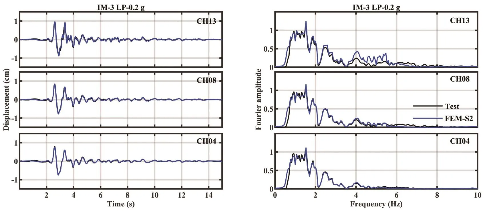
Fig.14 Comparisons between displacement results of STT and FEM, subjected to IM-3 (LP motion-0.2 g) at CH13, CH08 and CH04

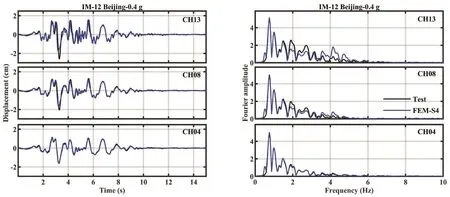
Fig.15 Comparisons between acceleration results of STT and FEM, subjected to IM-12 (Beijing motion-0.4 g) at CH13, CH08 and CH04

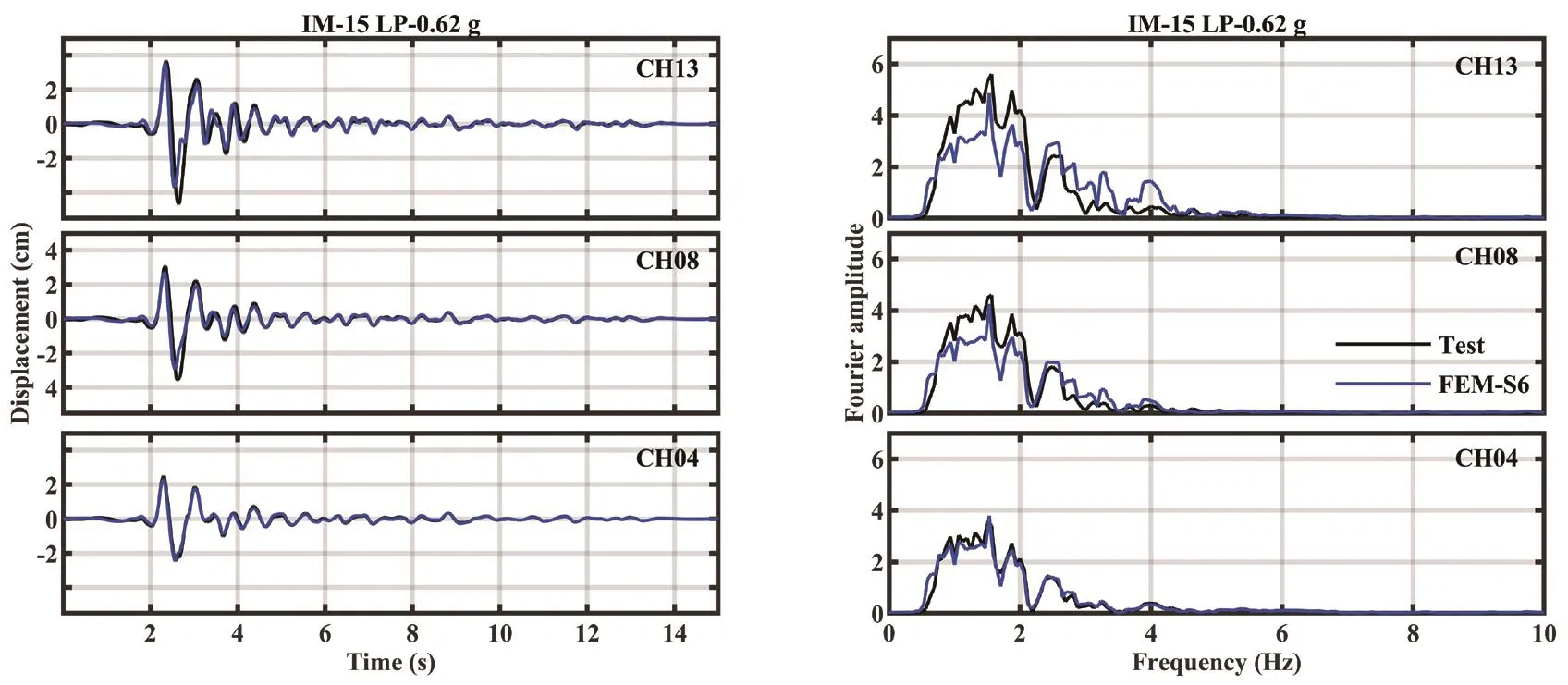
Fig.16 Comparisons between displacement results of STT and FEM, subjected to IM-15 (LP motion-0.62 g) at CH13, CH08 and CH04

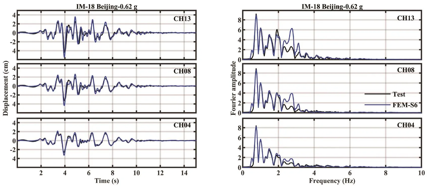
Fig.17 Comparisons between displacement results of STT and FEM, subjected to IM-18 (Beijing motion-0.62 g) at CH13, CH08 and CH04

5 Conclusions

1-g shaking table tests for a 3-m-height soil column were conducted.Typical experimental data were provided, and dynamic properties of three sand layers were estimated using results under the white noise, pulse and earthquake motions.Finite element modeling of the sand column was conducted to indirectly verify theestimated soil parameters.Conclusions can be drawn as follows:

1.The dynamic properties of the soil column were identified under white noise and pulse motions.The predominant frequencies of the sand were significantly reduced at the 0.2 g and 0.4 g stages, but they were steady after the 0.4 g stage.The viscous damping ratio of the sand column became amplified with the increasing peak acceleration of the input motions.

2.The maximum shear modulus and shear modulus degradation relationships of the three sand layers were characterized from 0.2 g to 1.0 g stages.The characterized parameters were effective and therefore could be used in numerical modeling to reproduce approximate seismic responses of the sand column.

Acknowledgement

This research was funded by the National Natural Science Foundation of China (52008233, U1839201),the National Key Research and Development Program of China (2018YFC1504305) and the Innovative Research Groups of the National Natural Science Foundation of China (51421005).We are thankful to Professor Gao Wensheng, the China Academy of Building Research,for providing a laminar shear box.We are thankful to Professor Chen Guoxing at the Nanjing University of Technology for the use of ABAQUS.We are thankful to Shen Yiyao, a student at the Beijing University of Technology, for his assistance on the shaking table tests.We are also thankful to Keshab Sharma and Austin Hong, students at the University of Alberta, for technical editing.