Less is more:a new machine-learning methodology for spatiotemporal systems

Sihan Feng,Kang Wang,Fuming Wang,Yong Zhang,2 and Hong Zhao,2

1 Department of Physics,Xiamen University,Xiamen 361005,China

2 Lanzhou Center for Theoretical Physics,Key Laboratory of Theoretical Physics of Gansu Province,Lanzhou University,Lanzhou 730000,China

Abstract Machine learning provides a way to use only portions of the variables of a spatiotemporal system to predict its subsequent evolution and consequently avoids the curse of dimensionality.The learning machines employed for this purpose,in essence,are time-delayed recurrent neural networks with multiple input neurons and multiple output neurons.We show in this paper that such kinds of learning machines have a poor generalization ability to variables that have not been trained with.We then present a one-dimensional time-delayed recurrent neural network for the same aim of model-free prediction.It can be trained on different spatial variables in the training stage but initiated by the time series of only one spatial variable,and consequently possess an excellent generalization ability to new variables that have not been trained on.This network presents a new methodology to achieve finegrained predictions from a learning machine trained on coarse-grained data,and thus provides a new strategy for certain applications such as weather forecasting.Numerical verifications are performed on the Kuramoto coupled oscillators and the Barrio−Varea−Aragon−Maini model.

Keywords:machine learning,spatiotemporal systems,prediction,dynamical systems,time series,time-delayed recurrent neural network

1.Introduction

Predicting the evolution of dynamic systems is important[1–3].These systems usually have to be solved numerically using spatial and temporal discretization because of the mathematical intractability of obtaining analytical solutions.In this way,a partial differential equation is approximated by a set of ordinary differential equations.The main obstacle to this approach is that it becomes infeasible in higher dimensions due to the need of fine-grained spatial and temporal mesh points,which is known as the ‘curse of dimensionality’[4].For real applications,one has to seek a balance between accuracy and computing cost by applying a relatively coarse mesh[1,5].The machine-learning approach developed in recent years provides possible ways to attack this notoriously difficult problem[6–9].One way is to solve partial differential equations with variables from randomly sampled grid points when the equation of motion is known.Researchers have developed an effective approach called physical informed neural networks[10]for this purpose.Another way,which is also the focus of this paper,is for application scenarios that have data records that are available for a large number of spatial points,while the equations of motion are unknown.A learning machine trained by the time series of such spatial points can predict their subsequent evolution in a model-free way[11,12].Using such a strategy,researchers from Google®developed a deep-learning machine called MetNet and improved local weather forecasts greatly[13].

In these applications,a recurrent neural network withQinput andQoutput neurons is employed to be the learning machine,whereQis the number of spatial variables whose time series records are used in the training.When training such a learning machine,the data from theQvariables are theQinputs,and the outputs represent the next-step evolution of these variables.Feeding the outputs back to the inputs,the learning machine can work as an iterative map.In this paper,we first check the generalization ability of such a learning machine applied to new sets ofQspatial variables that have not been trained with.This ability characterizes the robustness of the machine.For a real system,the system parameters may shift slightly as a function of time.As a result,the learning machine is expected to have a certain degree of robustness to such shifted data sets.Our numerical verification indicates,however,that such kind of learning machines have no such generalization ability.

To solve this problem,we propose,instead,to apply a one-dimensional(1D)time-delayed recurrent neural network as the learning machine to predict the evolution of the underlying system.In the training stage,the learning machine is still trained with time series collected from different spatial variables.In the predicting stage,however,the learning machine can be initiated by the history record measured at any one spatial point.We show that this learning machine can not only predict the evolution of the variables that have been trained with,but also that of variables that have not been trained with before.The advantages of such generalization ability are that the learning machine will be robust against small variations of system parameters,and it is possible to perform fine-grained predictions with a learning machine trained with coarse-grained data sets.This should be useful for applications such as the weather forecast as one can perform the prediction of a local region without the need of learning from the fine-grained mesh of the entire spatiotemporal system.Our numerical studies are performed on models of the Kuramoto coupled oscillators(KCO)[14–16]and the Barrio−Varea−Aragon−Maini equation(BVAM)[17,18].The rest of the paper is structured as follows.The machine-learning model and method are introduced in section 2.The main results are reported in section 3,in which the mechanism why the traditional approach has failed in transformational generalization while ours has succeeded is also explained.The summary and discussion are given in section 4.

2.Model and method

The learning machines adopted in this paper are schematically illustrated in figure 1.Figure 1(a)represents an MQ-N-Q neural network(with MQ,N,andQ,respectively,the number of neurons in the input,hidden,and output layer),or equivalently a Q-N-Q time-delayed map with a delay length ofM(as illustrated in the gray ellipse,Mneurons are utilized as the input units for each ofQinput records).Hereafter,it is called theQdimensional time-delayed machine(QD-TDM),of which the iterated map is given below:

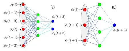
Figure 1.Schematic diagrams of the learning machines.(a)a 2-4-2 QD-TDM,with a delay length of M=3,and(b)a 1-4-1 1D-TDM,with a delay length of M=3.Each gray ellipse represents an input unit for time series from one spatial variable.

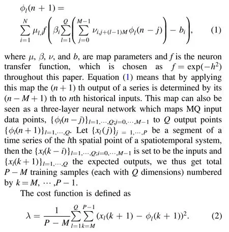
In the training stage,the cost function is minimized for theP−Mtraining samples under a properly chosen set of control parameters:M,N,Q,cμ,cν,cβ,andcb,and the last four specify the available ranges of the network parameters,i.e.,|μl,i|≤cμ,|νi,k|≤cν,|βi|≤cβ,|bi|≤cb.To perform the training,at fixedM,N,andQ,the μi,νi,k,βiandbiare randomly initialized in their respective value ranges,then a parameter from μi,νi,k,βiorbiis randomly chosen and then randomly mutated in its available range;this mutation is finally accepted if only that it does not increase the cost.Repeat the mutation step over and over again,the cost function will decrease monotonously.Since for each adaptation it needs to renew only a small portion of the network,this algorithm is practical for usual applications,see[19,20]for more details.Indeed,one can also apply the conventional gradient-based(also known as the back-propagation)algorithm to train our learning machine if removing the restrictions to the value ranges.Researchers in the machine learning community begin to try gradient-free algorithms in recent years,and the training algorithm presented here is one of such an effort.With this gradient-free algorithm one can achieve the goal of training,at least for the usual three-layer neural networks,while gaining the ability to limit the range of the network parameters,and therefore control the structural risk of the network.In addition,the parameters can take assigned discrete values,which may be required for certain practical applications.Under this background,we adopt our gradientfree algorithm instead of the conventional gradient-based algorithms.

In the predicting stage,one just needs to input the last samples ofk=Pto start equation(1),and feed the outputs back to the inputs correspondingly to make equation(1)a self-evolve iterate map.In the case of figure 1(a),for example,after the first round of iteration one needs to feedback φ1(t+3)to the up inputting unit,and φ2(t+3)to the bottom inputting one,and turns the inputs to φ1(t+1),φ1(t+2),φ1(t+3),and φ2(t+1),φ2(t+2),φ2(t+3),respectively,to initiate the second round of iteration.

Figure 1(b)represents an M-N-1 neural network,or equivalently a 1-N-1 time-delayed map with a delay length ofM(also illustrated in the gray ellipse).We will call it the onedimensional time-delayed machine(1D-TDM)afterwards,and its evolution dynamics are given by:

This equation appears as a reduced form of equation(1)as the summation of φlis replaced with a single φ.In the training stage,the time series of variables at multiple spatial positions are used sequentially to train the machine so that the dynamic information of those multiple spatial points are all learned by the machine.This is a key difference from previous strategies of training a 1D-TDM-like machine.In more detail,for thelth time series,set the{xl(k−i)}i=0,…,M−1to be the inputs and{xl(k+1)}the expected outputs,we again obtainP−Mtraining samples from one time seriesl.Apply the above operations to all of theQtime series and we get total(P−M)Qtraining samples(each in one dimension).The cost function has the same form as equation(2).In the predicting stage,only the last sample from one spatial variable is needed to initiate the learning machine.

We emphasize that those popular learning machines used for model-free prediction of the evolution of the underlying dynamic systems,such as the long short-term memory model[21]and the reservoir computer[22–25]are essentially equivalent to the time-delayed model described by the equation(1).The long short-term memory model manages a set of neurons in the hidden layers to memorize the history(i.e.,delayed information)of the inputted time series and thus is obviously equivalent to a time-delayed map.In using the reservoir computer,one needs to iterate the so-called reservoir for a sufficient number of steps before outputting the prediction in the initiation stage.The reservoir network indeed plays the role of storing the delayed information or memory.Thus,it is also a time-delayed map.Therefore,the QD-TDM can generally represent these conventional learning machines.

3.Results

3.1.The KCO model

We first test QD-TDM on the KCO model,which is given by

where ωiandK,respectively,represent the natural frequency and the coupling coefficient,andLis the total number of oscillators.We see from this equation that the motion of theith oscillator is determined not only by its natural frequency but also by the coupling from all other oscillators,with the strength being controlled by the parameterK.This model is widely applied to study the collective behavior of complex systems[15,16].With strong coupling,the oscillators may show synchronous oscillation and thus are reduced to an effective system with a low dimension.To avoid this case,weak coupling is applied to ensure that all of the oscillators oscillate roughly around their natural frequency ωiand the system lies in a weak chaotic state.The measurable variable of an oscillator is defined asx i(t)=sin(θi(t))+cos(θi(t))without loss of generality.

AtL=20 andK=0.8,we set ωiwith a random number from the interval(0,1).It can be checked that the system is chaotic with the largest Lyponov exponent being about 0.005.Evolving the system for a long time(with the time step of integralh=0.01)to collect a sufficiently long time series for each oscillator,then sample these time series with an interval of Δt=0.1 to construct the training set.We train the QDTDM using the first ten oscillators(i=1,2,…,10).The width of the learning machine is fixed atN=1000 throughout this paper,which is large enough for achieving the training goal.By searching the control parameter space we find thatM=2000,cμ=0.03,cν=0.45,cβ=0.05,andcb=40 to be the optimum control parameters for training the learning machine in the case of the KCO data set.After finishing the training,we first apply the learning machine to predict these first ten oscillators,and then apply it to evolve the next ten oscillators that have not been trained with(i.e.,inputting the time series from oscillators ofi=11,12,…,20 respectively to initiate the learning machine).

In figure 2(a),the black lines show segments of time seriesxi(t)fori=6 toi=15 as an example.The green and red lines show the predicted evolutions,for oscillators that have been trained with and for those that have not been trained with,respectively.We see that for the oscillators that have been trained with(i=6 toi=10),the predictions are quite good,but it totally loses the ability to predict for the oscillators(i=11 toi=15)that have not been trained with previously.

Then we use the same data of the first ten oscillators to train the 1D-TDM and apply it to predict all the 20 oscillators one by one.We find that not only the oscillators that have been trained with are well predicted,but those that have not been trained with previously are also well predicted to a large extent as can be seen in figure 2(b).Even using fewer oscillators to train this learning machine,the generalization ability is still considerable.Figures 2(c)and(d)show the results of the learning machine trained respectively by the oscillators ofi=1,2,3,4 and by only the oscillator ofi=1.It can be seen that,although the prediction quality gets slightly worse with the decrease of the number of training oscillators,the difference is not remarkable.Therefore,the 1D-TDM has excellent generalization ability to the new data set even trained by only few variables.

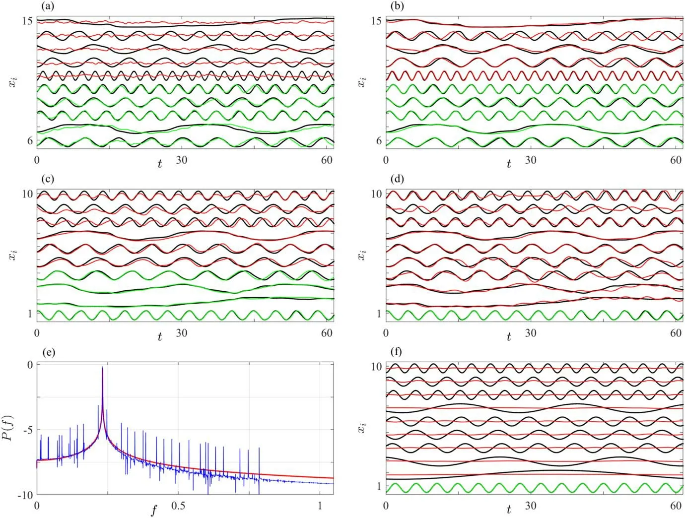
Figure 2.The generalization ability of QD-TDM and 1D-TDM to new variables for the KCO model.(a)Prediction results of QD-TDM trained with oscillators from i=1 to i=10,(b)–(d)prediction results of 1D-TDM trained with oscillators,(b)from i=1 to i=10,(c)from i=1 to i=4,and(d)with only i=1.The black lines represent data xi of the KCO model,and the green and red lines represent the predictions for oscillators that have been trained with(green)and for those that have not(red).(e)Shows,in semilogarithmic scale,the power spectrum of the first oscillator with control parameter K=0(red line)and K=0.1(blue line),and(f)shows the prediction of the 1D-TDM trained with the first oscillator(i=1)with K=0.

It is not surprising that a learning machine has the generalization ability to new variables that have not been trained on.According to the Takens theory,for a time series with a sufficient length,one can reconstruct anM-dimensional phase space map,whereMis the delay length.If onlyM>2D+1,this map should be topologically equivalent to the underlying dynamic system,whereDis the fractal dimension of the attractor of the underlying system.This is the well-known phase space reconstruction technique of delay-coordinate embedding[26,27].This theory holds because any variable of a dynamic system is considered to be coupled with others,and thus involves the information of other variables.

Figure 2(e)shows the power spectrum of the time series of the first oscillatorx1(t)withK=0(red line)andK=0.1(blue line),respectively.It can be seen that without coupling,the power spectrum only the frequency peak of this oscillator(red line).In this case,the learning machine involves no information of the other oscillators.It can be easily checked that the learning machine trained by this time series has no generalization ability to oscillators that have not been trained with previously,see figure 2(f).With a non-vanishing coupling,it is seen that though it is difficult to observe the coupling effect of other oscillators by just looking at the evolution curve(see black lines figure 2(d)),the power spectrum actually includes frequency peaks of the other oscillators(see the blue line in figure 2(e)).These peaks have a very small amplitude(note that the vertical axis is with the logarithmic scale),and differ among different oscillators.The power spectrum confirms that the information of other oscillators are coupled to the first oscillator,which provides the basis that the learning machine trained by data of only one of the oscillators could have the generalization ability to other coupled ones.

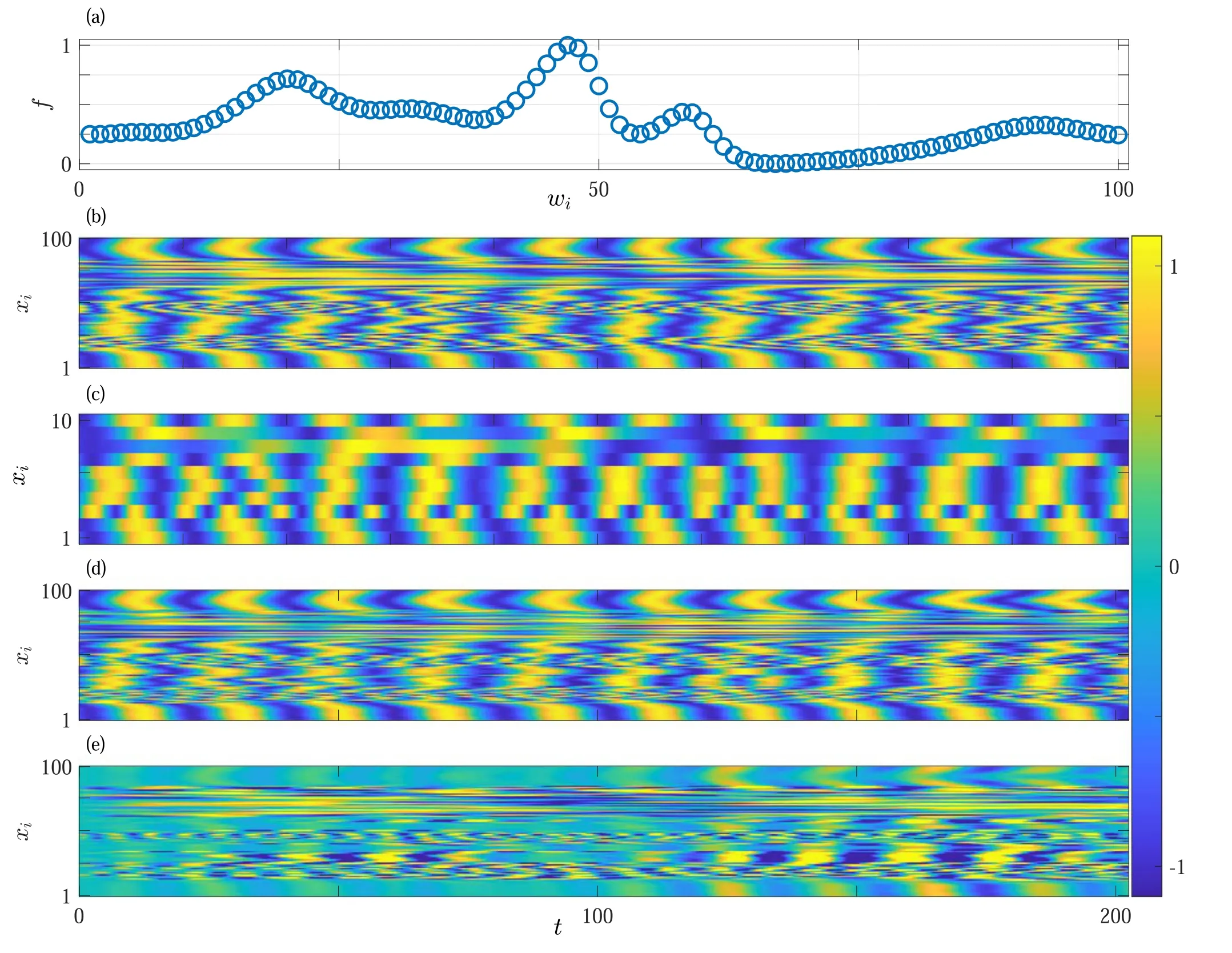
Figure 3.Recovering fine-grained spatiotemporal structures of the underlying system using the 1D-TDM trained with small portions of the variables.(a)ωi of oscillators,(b)actual fine-grained spatiotemporal pattern of the KCO model,(c)predicted coarse-grained spatiotemporal pattern of the KCO model.(d)Fine-grained spatiotemporal pattern recovered by the 1D-TDM.(e)Prediction errors(panel(b)minus panel(d)).

The phase space can also be reconstructed using multiple time series with the technique of delay-coordinate embedding[27].The reason why a 1D-TDM can,while a QD-TDM cannot be applied to spatial points that have not been trained with previously is the following.A remarkable different property of the 1D-TDM from the QD-TDM is that it does not involve the time unit explicitly in its equation of motion;what is inputted to the learning machine is just a discrete time series[see equation(3)].With this feature,a 1D-TDM can evolve the dynamics of any oscillator once it is initiated by its time series if only the information of this oscillator is correctly coupled into the learning machine.In contrast,theQtime series with different frequencies are needed to be evolved simultaneously in a QD-TDM(see equation(1)),which thus introduces a relative time unit to the machine.If,for example,it is trained by two time series with frequencies ω1and ω2,then a relative time unit is defined by the ratio of ω2/ω1.The learning machine could correctly recover the dynamics of two oscillators with frequenciescω1andcω2,if these two oscillators belong to the underlying system.In this case,the time series of ω1and ω2and the time series ofcω1andcω2have the same relative time unit.However,if the learning machine is applied to a new set of oscillators with ω3and ω4,the relative time unit changed,and mismatching arises.The mismatching may become more serious for largerQ.

This generalization ability of the 1D-TDM provides a useful strategy for possible applications to perform finegrained predictions using a learning machine trained on coarse-grained data.To show such a possibility,we construct a KCO model with 100 oscillators.The oscillators take frequencies following the curve shown in figure 3(a).Setting the frequencies in such a way,the KCO model can exhibit finegrained evolution patterns as shown in figure 3(b)instead of random patterns.Using 10 evenly spaced oscillators to train a 1D-TDM,we find that it can recover the subsequent evolution of these 10 oscillators well,which gives a coarse-grained picture of figure 3(b)in figure 3(c).However,using the trained learning machine to predict every oscillator,we recover figure 3(b)approximately in figure 3(d).Figure 3(e),shows the prediction errors,indicating that the recovery is almost perfect in a long period of an earlier time;the errors increase with the further increase of time,but they are overall relatively small compared to the original variable,demonstrating an excellent prediction ability of the machine.

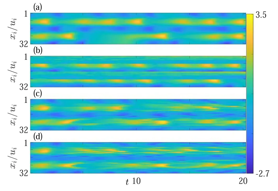
Figure 4.The generalization ability of QD-TDM and 1D-TDM for the BVAM model.(a)Spatiotemporal patterns of the model with the spatial variable u.(b)Predictions of the QD-TDM trained with mesh nodes of i=9,10,…,16.(c)and(d)are the predictions of the 1DTDM trained with mesh nodes of i=9,10,…,16 and i=1,3,5,7,9,respectively.

3.2.The BVAM model

In the KCO model,the amplitudes of oscillators are identical and oscillators are coupled globally.In this case,the time series of any oscillator may fully involve the information of all oscillators.Therefore,the 1D-TDM trained by only the time series of one oscillator may recover the dynamics of all the other oscillators.In other systems,the coupling among different variables may be different and may only couple locally.In this case,however,one has to involve more time series of representative spatial variables to train the learning machine to gain a better generalization ability to other variables.To show this,we study another spatiotemporal system,i.e.,the BVAM model,whose equations of motion are given by

whereC,D,H,η,a,andbare system parameters.This model presents the richness of dynamic behavior[18].Fix the system size atLb=6.4 with 32 mesh nodes for bothuandv,and solve the equation(5)numerically(with the time step of integralh=0.01)in one dimension with zero flux boundary conditions and random initial conditions around the equilibrium point(0,0),atD=0.08,H=3,η=1,a=−1,b=−3/2,andC=−1.54.The evolution of time is shown in figure 4(a),from where typical chaotic spatiotemporal patterns appear,i.e.,spatial variables oscillate chaotically with the evolution of time.Typically,it can be seen that the oscillation range is different in different regions,manifested by the bright-yellow and dark-blue colors.

Sample the time series of the mesh nodeui(t)at an interval of Δt=0.1 and obtain the measurable time seriesxi(t).For this system,the optimum set of control parameters areM=300,cμ=0.02,cν=1,cβ=0.5,andcb=30.Using data ofxi(t)/ui(t)withi=9,…,16 to train the QD-TDM and the 1D-TDM respectively and then apply them to produce the evolution of the whole system after finishing the training,and the results are shown in figures 4(b)and(c),respectively.It is seen again that the QD-TDM can recover the dynamics of the spatial variables that have been trained with but not to the ones that have not(see figure 4(b)).The 1D-TDM,in contrast,possesses the ability to predict time evolution of variables in the spatial regions that have not been used for training(see figure 4(c)).Since this is a relatively strong chaotic system,the predictable time region is relatively shorter than in the case of the KCO model.

Choosing mesh nodesxi(t)/ui(t)withi=1,3,5,7,9 to be the training time series,the 1D-TDM can still recover the evolution dynamics of the whole system in figure 4(d).Even using only three mesh nodesxi(t)withi=1,which represents variables in the dark-blue region,i=9,which represents those in the bright-yellow region,andi=5,which represents those in the light-green region,the 1D-TDM still retains some ability to generalize.When using the data from only one spatial variable,the generalization ability remains to some extent for spatial variables that belong to the same class,but not for the other classes.

4.Summary and discussions

In summary,the usual recurrent learning machine,requiring multiple system variables to iterate,almost has no generalization ability to the ones that have not been trained with previously.Applying such a learning machine,the number of sampled variables has to be sufficiently large to cover the major modes of the system,and predictions are only available for those variables that have been trained with.Meanwhile,using the 1D time-delayed map as the learning machine can predict the subsequent evolution of not only variables that have been trained with,but also variables that have not.Specifically,this learning machine requires data from only one variable to iterate,it can be trained with a small set of variables,and it can predict the evolution of the small set of variables it trained with as well as other variables that it did not train with.One of the possible applications of this property is that we may,after being well-trained,apply the learning machine to densely sampled spatial variables in a local region and thus gain the fine-grained evolution patterns of this region.This finding provides a new strategy for special applications such as weather forecasting,where high-resolution prediction may be obtained for a local region using a learning machine trained on low-resolution data from the same region.Presently,this strategy is just illustrated for relatively simple spatiotemporal systems.We hope a more systematic approach can be developed to treat real-life spatiotemporal systems in the future.

Acknowledgments

We acknowledge support from the NSFC(Grants No.11 975 189,No.11 975 190).