Ship Local Path Planning Based on Improved Q-Learning

-,-,,,-

(1.Key Laboratory of High Performance Ship Technology(Wuhan University of Technology),Ministry of Education,Wuhan 430000,China;2.School of Transportation,Wuhan University of Technology,Wuhan 430000,China)

Abstract:The local path planning is an important part of the intelligent ship sailing in an unknown en⁃vironment. In this paper, based on the reinforcement learning method of Q-Learning, an improved QLearning algorithm is proposed to solve the problems existing in the local path planning, such as slow convergence speed, high calculation complexity and easily falling into the local optimization. In the proposed method, the Q-table is initialized with respect to the artificial potential field, so that it has a prior knowledge of the environment.In addition,considering the heading factor of the ship,the two-di⁃mensional position information is extended to the three-dimensional by joining the angle information.Then,the traditional reward function is modified by introducing the forward information and the obsta⁃cle information obtained by the sensor,and by adding the influence of the environment.Therefore,the proposed method is able to obtain the optimal path with the ship energy consumption reduced to a cer⁃tain extent. The real-time capability and effectiveness of the algorithm are verified by the simulation and comparison experiments.

Key words:Q-Learning;state set;reward function

0 Introduction

Path planning plays an important role in navigation of the autonomous vehicles like unmanned surface vehicle (USV). The path planning methods include the global path planning and the local path planning.In the global path planning,the safe path is planned for the USV under a static envi⁃ronment,where the obstacles are assumed to be known.The local path planning deals with the prob⁃lems of identifying the dynamic condition of environment and avoiding obstacles in real time. For the local path planning, some algorithms have been proposed in the literature, such as the artificial potential field[1], genetic algorithm[2], fuzzy logic[3], neural network[4-6]and so on. These algorithms can plan a safe path under the partially known environment or some unknown environment.But the adaptability of these algorithms for the unknown environment or mutation environment is not very well.

At present, the reinforcement learning is the hottest research area. There are many studies about reinforcement learning on path planning[7-9]. Common reinforcement learning algorithms in⁃clude Q-Learning,SARSA,TD-Learning and Adaptive Dynamic Planning.Sadhu[10]proposed a hy⁃brid algorithm combining the Firefly algorithm and Q-Learning algorithm. In order to speed up the convergence, the flower pollination algorithm was utilized to improve the initialization of Q-Learn⁃ing[11]. Cui[12]optimized the cost function through Q-Learning to obtain the optimal conflict avoid⁃ance action sequence of UAV under the motion threat environment, and considered the maneuvers in order to create the path planning that complies with UAV movement limitations.Ni[13]proposed a joint motion selection strategy based on tabu-search and simulated annealing,and created a dynam⁃ic learning rate for the path planning method based on Q-Learning so that the method can effective⁃ly adapt to various environments.Ship maneuverability is integrated in Q-Learning algorithm as pri⁃or knowledge,which shortens the model training time[14].

In this paper, we propose an improved Q-Learning algorithm for the ship sailing in an un⁃known environment. Firstly, this algorithm increases the state variable and includes the ship’s heading information,so that it can increase the path smoothness,and also changes the number of ac⁃tions to increase the path diversity. Then, we introduce the potential field gravity to initialize the Q table to speed up the convergence of the algorithm. After that, we modify the reward function, by adding the angle of environmental force and the forward guidance to the target point, to reduce the exploration step number and the calculation period of the algorithm. The search performance of the traditional algorithm and that of the improved algorithm in different environments are compared in the simulation experiments respectively.

1 Classical Q-Learning algorithm

Q-Learning is a typical reinforcement learning algorithm developed by Watkins[15], and it is a kind of reinforcement learning without environment model. Q-Learning applies the concept of reward and penalty in exploring the unstructured environment, and the term of Q-Learning is shown in Fig.1. Agent in the Fig.1 represents the unmanned vehicle, and in this paper, it repre⁃sents USV.State is the position of USV in local environment,and action is the movement that the USV moves from current state to next state.For the reward,it is a positive value to increase the Q-value for the cor⁃rect action. Besides, the penalty is a negative value to decrease the Qvalue for the wrong action.

In general,the idea of Q-Learning is not to estimate an environment model,but to directly op⁃timize a Q function that can be iterated.The policy being applied is not affected by the values of the optimal Q to be converged. TheQvalues of the Q-Learning algorithm is updated using the expres⁃sion:

Fig.1 Interaction between agent and environ⁃ment

wheresindicates the current state of ship,aindicates the action performed insstate,rindicates the received reinforcement signal aftersexecuted,γindicates the discount factor (0＜γ＜1), andαindi⁃cates the learning coefficient(0＜α＜1).

TheQvalue of the next possible state is determined by the following expression:

whereεindicates the degree of greed,and it is a normal number with the values between 0 and 1,cis a random value,andArepresents the set of actions.

2 Improved Q-Learning algorithm

2.1 Improved state set

The state in the traditional Q-Learning algorithm is represented by the grid position, and the corresponding four actions of each state are up,down,left and right[16].However,the ship path plan⁃ning not only needs the position information, but also needs to consider its heading information.Therefore, the following improvements are made in this paper: (1) the angle information introduced on the basis of the position information is discretized into eight directions. In other words, the state is extended from two degree of freedom (DOF) to three DOF, as shown in Fig.2; (2) four additional actions are introduced, i.e., left front, right front, left back and right back, as shown in Fig.3; with the increase of action set, the planned path is more diverse than the traditional method. Besides, in this paper, some actions are punished, such as the back action, because the ship cannot perform a large bow turn and is less likely to perform a retreat.

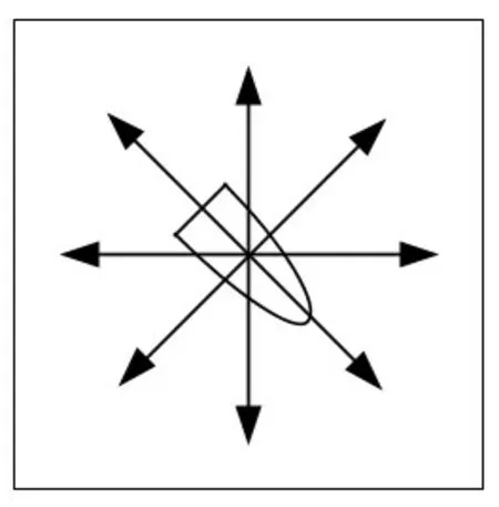
Fig.2 Improved status

Fig.3 Improved action

The ship motion coordinate system established is s hown in Fig.4, in whichθvrepresents the ship heading,θgoalrepresents the angle between the ship’s current position to the target point and thexax⁃is,andθenvrepresents the direction of the environmental force.

In order to quantitatively analyze the degree of path smoothness planned by the algorithm, a path angle function is introduced as follows:

whereθi-θi-1indicates the included angle between the pointiand its previous point,nrepresents the number

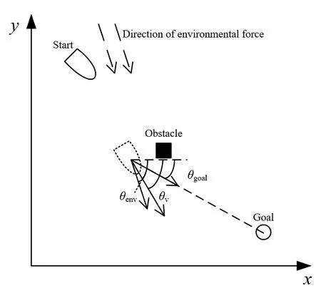
Fig.4 Ship motion coordinate system

of path points. Obviously, the smaller the value ofζ, the smoother the path curve, which is more suitable for ship navigation.

2.2 Prior information

We know that the artificial potential field method is widely used in path planning. Its basic idea is to construct an artificial potential field in the surrounding environment of a ship, which in⁃cludes the gravitational field and the repulsive field. The target node forms a gravitational field to the ship, and the obstacle has a repulsive force field in a certain range around it, which makes the joint force in its working environment push the ship forward to the target. The traditional Q-Learn⁃ing algorithm has no prior information,which means that theQvalue is set to a same value or a ran⁃dom value in the initialization process, so the convergence speed of the algorithm is slow. In order to solve the above problems,the gravity information of potential field is introduced when theQtable is initialized. That means we add the environmental prior knowledge to speed up the convergence of the algorithm.

The gravitational function is defined as

2.3 Improved reward function

The reward function in Q-Learning maps the perceived state to the enhancement signal to evaluate the advantages and disadvantages of the actions. The definition of the reward function de⁃termines the quality of the algorithm. The traditional Q-Learning algorithm has a simple definition of return function and does not contain any heuristic information,which leads to a slow convergence speed and high complexity of the algorithm. In this paper, the reward function is divided into three stages:reaching the target point,encountering obstacles and the stage showed in Eq.(6).

wheref1,f2,andf3are the predefined numbers,pis the current point,Goal is the target point,dobsis the obstacle position,dois the obstacle influence range,m1,m2andm3are the weight coefficients,which are positive, and the sum of them is 1,d1,d2, andd3are the evaluation factors defined as fol⁃lows:

whered2is the angle evaluation factor,andk1andk2are the weight coefficients.It can be seen from Fig.4 that when the ship implements the collision avoidance measures with the influence by envi⁃ronmental force at the same time, the direction of the environmental forces is quite relevant to the direction of the ship, which means it should follow the direction of environmental resultant force,which is beneficial to the saving of energy. Suppose the angle between the direction of the environ⁃mental force and the direction of the ship is between 120°and 240°,it is relatively energy-consum⁃ing.So it is necessary to combine the angle between the heading and the target position,the smaller the angle,the better.In that course of the ship,the direction of navigation is the same as that of the environmental force, which is beneficial to energy conserving. However, at the same time, the state of the target point cannot be excessively deviated, so the punishment will be larger when the devia⁃tion angle of the ship is higher.

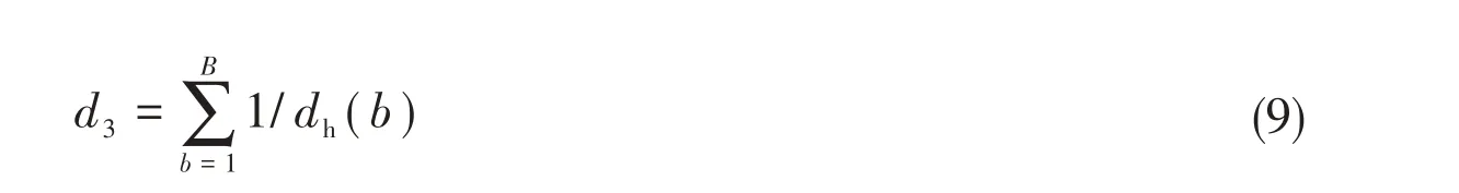
whered3is the obstacle evaluation factor,bis the total number of obstacles in the sensor detection range, and thedh(b) is the distance from the current point to the obstacle position. The formula shows that the closer the ship to the obstacle,the greater the penalty.

Due to the heading of the ship is limited and we do not want the ship to retreat. For example,the ship moves from one state to another,but the action is not front,left front or right front,so the in⁃centive value is set to a negative value to avoid a large change in the path angle planned by the algo⁃rithm.

2.4 Modification of greedy selection

The balance between the exploration and exploitation of the algorithm depends on the greedy setting,and the greed of the traditional algorithm is set to a constant,which makes the algorithm de⁃pend on the quality of the set value. If the setting value is too large, the algorithm will fall into the local optimal that cannot jump out.If the setting value is too small,the algorithm will still find other paths,even the smallest path,resulting in a slow convergence speed and a long calculation time.In this paper,we propose an adaptive greed.The algorithm pays attention to the path exploration in the early stage to improve the path diversity. With the increase of the number of iterations, the algo⁃rithm focuses on the exploitation of the results of the previous exploration,and the formula is as fol⁃lows:

wherehis the current number of iterations andεmaxis set to the maximum greedy value. As can be seen from Eq.(10),with the increase of the number of iterations,the greedy value increases until the maximum value is reached.Therefore,the probability of the random selection action is gradually re⁃duced,and the converge of the algorithm is accelerated.

2.5 Algorithm pipeline

The improved algorithm pipeline is shown in Fig.5,and is described as follow:

Step 1: Establish aQtable formed by state and action, and initialize theQvalue table, the start stateSand the iterative counterh,and the stateSis a three-DOF information composed of the grid position and the angle to determine whetherSis the target point.

Step 2: At the beginning of the iteration, the greed degreeεis set according to Eq.(10) in the action policy selection. If the random valuecis less thanε, then randomly select the action. If the random valuecis larger thanε,then select the action of the maximumQvalue according to Eq.(2).

Step 3: Select the reward value of the action according to Eq.(6), and the determination of its reward value contains the direction of environmental force, whether to advance to the target point and the distance from the obstacle.

Step 4: Update theQvalue table according to Eq.(1). If the next state is the target, the loop ends, otherwise, turn back to Step 2. If the result of the successive 15 iterations is consistent, the output result is considered to be converged in advance, otherwise, if the number of iterationshis greater than 1000,the result is outputted directly.

Fig.5 Flow chart of the improved Q-Learning algorithm

3 Simulation results and analysis

In order to verify the validity of this algorithm,the improved Q-Learning algorithm and the tra⁃ditional Q-Learning algorithm are compared under the simulation platform of Python 3.6 with CPU of Intel (R) Core (TM) i3, 3.9 GHz, and 8 G memory. The grid map is established and the sensor measurement range is set to four girds, as shown in Fig.6. The simulation situation is divided into two common scenarios:one is that there are many obstacles at the starting point of the ship when en⁃tering the port, and the other is that there are obstacles at the target point when the ship leaves the port. One of the maps is a grid with a small map of 10×10, and the other is a grid with a large map of 20×20.The related parameters set in the algorithm are as follows:the maximum number of itera⁃tionsh=1000, the learning rateα=0.4, the discount factorγ=0.95, the greedy policyε=0.5,εmax=0.95,the parameters ofm1,m2andm3are 0.7,0.2 and 0.1 respectively,and those off1,f2,f3are+10,-10,-0.02.If the same value is outputted for 15 consecutive rounds,it can be regarded as the con⁃vergence of the algorithm in advance, otherwise the algorithm ends when the number of iterations reaches the maximum.

Fig.6 Simulation environment

Fig.7 and Fig.8 show the path lengths of the two algorithms in the small map and the large map respectively,where Fig.7(a)and Fig.8(a)are the traditional algorithms and Fig.7(b)and Fig.8(b)are the improved algorithms. As can be seen from Fig.7, the maximum number of exploration steps of the traditional algorithm is 1600 steps while that of the improved algorithm is only 15 steps, which is reduced by 99.06%. When the map becomes larger, the number of exploration steps increases.The number of exploration steps in the early stage of the traditional algorithm is larger than that of the latter, and most of them are above 500 steps, with a maximum of 3000 steps. Compared with that of the traditional algorithm, the number of exploration steps of the improved algorithm is pretty small, and the highest is 32 steps, only 1.07% of that of the traditional algorithm. So, we can con⁃clude that the improved algorithm performs better in exploration performance than the traditional al⁃gorithm.

Fig.7 Length of path versus the iterations in small map

Fig.8 Length of path versus the iterations in large map

Fig.9 and Fig.10 are the path graphs of the two algorithms under the small map and large map,where Fig.9(a) and Fig.10(a) are the traditional algorithms, and Fig.9(b) and Fig.10(b) are the im⁃proved algorithms. From Fig.9, we can see that the improved algorithm increases the action set and improves the diversity of paths.In addition,the improved algorithm converts the two-DOF variables of the state into the three-DOF by adding the information of heading,and considers the limitation of ship motion.As can be seen from Fig.10,the improved algorithm reduces the rotation angle and im⁃proves the smoothness of the path.

Fig.9 Planned path in small map

In Fig.9, there are more obstacles at the end point, however, in Fig.10, there are more obsta⁃cles at the starting point,which is similar to the cases of the ship entering and leaving port.We can see that the improved algorithm can plan a better route from the starting point to the target node.

Fig.10 Planned path in large map

Tab.1 shows the comparison of the performance of the above-mentioned algorithm in the path planning, including the important factors such as running time, total running steps, path length and angle. Meanwhile, we average the data in the table after 10 times of operation. In the simple envi⁃ronment, compared with that of the traditional algorithm, the total operation step size of the im⁃proved algorithm is reduced by 91.19%,and the final path is shortened by 38.89%.Meanwhile,the smoothness of the planning path is increased 79.17%, and the time is shortened by 83.22%. In the complex environment, the step size of the improved algorithm operation is reduced by 98.59%, the path length is shortened by 42.11%, the path smoothness is improved by 75%, and the time is re⁃duced by 95.98%. The simulation results show that the improved algorithm is superior to the tradi⁃tional algorithm.And when the map is enlarged,the time of the improved algorithm is less than that ofthe traditional algorithm,indicating its effectiveness and real-time performance.

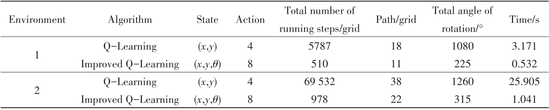
Tab.1 Performance comparison of different algorithms in different environments

4 Concluding remarks

This paper presented an improved Q-Learning algorithm for the local path planning of an un⁃known environment.In the proposed algorithm,theQvalue table was initialized with potential field gravity to reduce the number of exploration steps. The two-DOF state variable was extended to the direction information of three-DOF with a reduced curvature of the route. The path was diversified by adding action set while angle limit was considered to meet the requirements of ship driving at the same time. Such information as the reward function, the introduction distance and the environment force direction was modified,with the convergence speed of the algorithm accelerated and the path length shortened as a result. Comparison of the traditional Q-Learning algorithm with the improved algorithm and the simulation results show that the improved algorithm is effective and feasible.