Flow field fusion simulation method based on model features and its application in CRDM
2022-05-12SiTongLingWenQiangLiChuanXiaoLiHaiXiang
Si-Tong Ling · Wen-Qiang Li· Chuan-Xiao Li · Hai Xiang
Abstract The control rod drive mechanism(CRDM)is an essential part of the control and safety protection system of pressurized water reactors. Current CRDM simulations are mostly performed collectively using a single method,ignoring the influence of multiple motion units and the differences in various features among them,which strongly affect the efficiency and accuracy of the simulations.In this study,we constructed a flow field fusion simulation method based on model features by combining key motion unit analysis and various simulation methods and then applied the method to the CRDM simulation process. CRDM performs motion unit decomposition through the structural hierarchy of function-movement-action method, and the key meta-actions are identified as the nodes in the flow field simulation. We established a fused feature-based multimethod simulation process and processed the simulation methods and data according to the features of the fluid domain space and the structural complexity to obtain the fusion simulation results. Compared to traditional simulation methods and real measurements, the simulation method provides advantages in terms of simulation efficiency and accuracy.
Keywords CRDM · Flow field simulation · Motion unit analysis · Simulation method fusion
1 Introduction
Nuclear energy has become the focus of energy research in various countries because of its cleanliness and efficiency [1-3]. The control rod drive mechanism (CRDM)shown in Fig. 1 is a motion device used to regulate the reaction power in the reactor of a nuclear power plant.The CRDM is arranged inside the pressure vessel, and its motion is influenced by the core coolant. For safety reasons, the CRDM needs to quickly respond to commands during operation,and the resulting changes in the flow field affect its motion properties and reduce the accuracies of the motion pattern and timing. Therefore, a simulation of the flow field around the CRDM is needed to investigate and understand the relationship between them and degree of influence of the flow field on the CRDM. CRDM motion requires the support of many components that cooperate with each other to form several structural units of motion.To obtain comprehensive flow field information, the motion process of different structural units must be simulated together. However, the overall simulation is a timeconsuming task, and the simulation results obtained using different methods for the same characteristic unit may differ. Therefore, efficient and accurate simulation of complex CRDMs has become a key issue for the effective use of nuclear energy.
Recently, researchers have conducted numerous studies on the simulation and analysis of the flow field during CRDM motion. Lee et al. [4] studied the connection point between a CRDM and pressure vessel and analyzed theeffect of fluid stress on the weld position. Babu et al. [5]developed a mathematical model of the dynamic characteristics of a CRDM during an emergency shutdown and calculated the relationship between each drag force and the influencing factors during the control rod drop.Yu et al.[6]numerically simulated the three-dimensional flow field of a servo-piston CRDM and obtained the pressure distribution of the flow field inside the cylinder and flow characteristics of the throttle. The control rod is buffered to varying degrees by changing the size of its flow path,fluid pressure,and outlet flow rate during the drop [7-9]. Qin et al. [10]analyzed the structural components and operating principles of a new hydraulic CRDM and simulated the fluid domain within the drive system during the control rod drop.Liu et al. [11] proposed an iterative method for flow field analysis of the drop process of control rods,where the flow state, pressure distribution, and fluid resistance are solved by calculating the flow energy loss and integrating all flow states into a set of Bernoulli and conservation equations.Xiao et al. [12] simulated the three-dimensional flow field of the falling process of a single control rod using the dynamic mesh method and obtained pressure and velocity distribution diagrams of the flow field in the guide tube,as well as displacement-time and velocity-time curves.These researchers explored the flow field by treating the CRDM as a whole, without specifying the effect of the different motion units within it on the flow field.Therefore,the flow field simulation model contains many unimportant structures, and the simulation is not efficient. In addition, these authors only used a single method in the simulation and did not compare the simulation results of different methods,so simulation accuracy could not be verified.

Fig. 1 Structure of reactor and CRDM
The inflow method (IM) and dynamic mesh method(DMM) are the two most commonly used flow field simulation methods. The IM treats the moving object as stationary and makes the fluid around the object flow toward the object at the velocity at which the object is moving.This converts the solution of a moving object into a solution of a moving fluid through the principle of relative motion.The IM is widely used in the engineering field because its use and calculations are easy [13-17]. The DMM preserves the motion properties of the object and simulates fluid changes during object motion by updating the mesh state in the computational domain in real time.Simulations using DMM require keeping the object in motion for a period, so the method can support the simulation of variable-speed motion and obtain the flow field state at the end moment of the motion process. DMM has been applied extensively in engineering fields, such as simulating motion state of aircrafts and submersibles[18, 19], studying the aerodynamic characteristics of highspeed trains[20],and analyzing fluid motion state[21,22].DMM has also been applied for atomic layer deposition motion simulation [23], fish swimming characteristics calculation [24], and blood flow state study [25]. Because of the reverse in computational principles, flow field simulations using the IM and DMM yield different, even considerably discrepant, results. As such, the applicability of both methods and the features of the simulation model must be combined to select the appropriate method for each type of simulation data.
In summary, two problems exist in the current research on the flow field of CRDMs. First, for the multiple motion units of a CRDM,researchers have only conducted overall analyses without the selection of key motion units, resulting in a simulation process that consumes a large amount of computational resources and has low simulation efficiency.Second, for the many features of the CRDM simulation model, only a single method has been used for simulation,lacking targeted simulation method selection for different features, leading to inaccurate calculation results. Therefore,using CRDM as the research object,in this study,we aimed to construct a flow field fusion simulation method based on model features. By decomposing the CRDM using the function-movement-action (FMA) structural hierarchy, we proposed to obtain a collection of meta-actions and identify the meta-actions with a high degree of influence on the flow field as nodes for the simulation.We established a feature-based IM-DMM fusion simulation process and discretized the simulation model of the drive mechanism into features. We selected applicable simulation data for two main simulation features: fluid domain space and structural complexity. We improved each simulation method according to the selection and performed simulations separately. We extracted the required data from the simulation results for each feature and obtained the results by fusing the simulation data in the order of the features.
2 Determination of key motion structural units based on FMA
The parts of the CRDM always cooperate to complete complex functions and motions. At different motion time nodes, the parts involved in the work and their motion states are different, which diversifies the flow field of the CRDM. Therefore, the motion nodes that must be simulated should be determined before the flow field simulation.In this study, we structurally decomposed the CRDM according to its function and motion and obtained a set of meta-actions that can reflect each motion.Among them,we selected the action element that strongly affected the flow field as the simulation node to improve the efficiency of the simulation.
2.1 FMA analysis of motion structure unit
Meta-action is the basic constituent element in the movement process of a mechanical system and is responsible for power transmission between various parts of the system [26]. A complex mechanical system can be decomposed into several independent meta-actions from the function perspective. By integrating the parts participating in the meta-action according to a certain structural relationship, an independent meta-action unit can be formed [27]. Figure 2 shows the composition and connections of a meta-action unit. The function of the CRDM involves several meta-actions as a collection of complex structures.To perform a systematic and structured analysis of the various functions and motions of the CRDM, the movement process must be decomposed. And the simulation node is determined based on the results of the analysis.In FMA motion structure unit analysis, the hierarchical FMA relationship is used to analyze the complex system layer-by-layer in a single direction and finally to describe the entire system through a set of meta-actions [28]. We performed the following hierarchical decomposition of CRDM using this method:
(1) Determination of a function layer The core functions of the CRDM include adjusting the reaction power,replacing the fuel assembly, and stopping the reaction.Denoting CRDM and these three functions as S,F1,F2,and F3, then S = {F1, F2, F3}.
(2) Determination of a motion layer CRDM always performs in a stepwise manner when lifting and inserting control rods, requiring the coordination of the components that provide the stepping motion and the maintenance of the stepping state.Based on this feature,the components of CRDM can be divided into stepping and holding assemblies. Therefore, the motion of the CRDM can be divided into stepping assembly ascending, stepping assembly descending, holding assembly ascending, and holding assembly down,which are denoted as M1,M2,M3,and M4,respectively. The functions of power adjustment F1and fuel replacement F2require all the motions to be involved,that is, {F1, F2} = {M1, M2, M3, M4}. The reaction stop function F3only needs the support of the stepping component ascending M2and the holding component ascending M4, that is, F3= {M2, M4}.
(3) Determination of the action layers The stepping assembly includes lifting the armature, moving the armature, and moving the latch, and the holding assembly includes holding the armature and holding the latch. By combining the meta-motion of the base parts, the liftinginsertion motion of the stepping assembly and holding assembly can be accomplished. The meta-actions of these parts include the moving armature movement, lifting armature movement, moving latch rotation, holding armature movement, holding latch movement, and drive rod movement,which are denoted as A1,A2,A3,A4,A5,and A6, respectively. The corresponding meta-action units are denoted as U1, U2, U3, U4, U5, and U6, respectively. The ascent and descent of the stepping component require the rotation of the moving latch and movement of the moving armature, lifting armature, and drive rod. That is, {M1,M2} = {A1, A2, A3, A6}. Similarly, the ascent and descent of the holding component require rotation of the holding latch and movement of the holding armature. Thus, {M3,M4} = {A4, A5}.
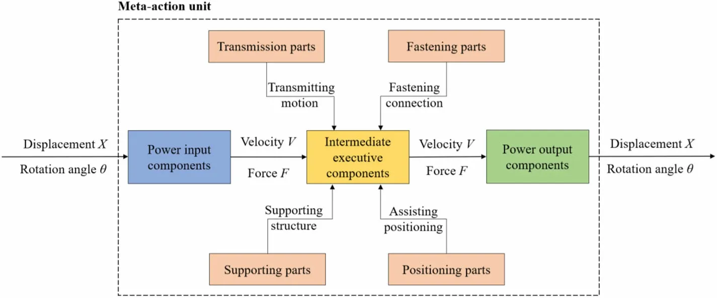
Fig. 2 (Color online)Composition and connection of the meta-action unit
Finally, the FMA structure decomposition diagram of the CRDM was drawn according to the decomposition results of each layer (Fig. 3).
2.2 Determination of key motion structural units
In simulations of the flow field around a CRDM, the focus is the fluid resistance of the mechanism and disturbance of the flow field. The fluid resistance is affected by the speed of the object and its contact area with the fluid along the direction of motion [29]. The disturbance of the flow field is related to the volume of the object and complexity of the parts.
The CRDM is driven by a larger force in the upward process than in the downward process, and its movement speed is similar. This causes higher fluid resistance during the upward movement and more violent flow field disturbances. For the area in contact with the fluid along the direction of movement, we ordered the six meta-action units as U2>U1>U4>U6>U3≈U5and ordered the fluid resistance in a similar manner. We ordered the structural volumes as U2>U6>U1>U4>U3≈U5. A unit with a larger volume causes increased fluid flow during movement, resulting in a stronger disturbance.Quantitatively determining the complexity of these parts is difficult. However, the drive rod can be visualized as having a large number of annular grooves and the latches containing anisotropic structures [30]. Compared to the armature, these two parts produce more complicated disturbances in the flow field.
Because the lifting armature always moves with the moving armature, moving latch, and driving rod during upward movement, we integrated the meta-actions of the three into the lifting meta-action set AS1-2-3-6, which corresponds to the lifting meta-action unit set US1-2-3-6.Likewise, the moving armature is linked to the moving latch during the upward movement,and the meta-actions of both form the moving meta-action set AS2-3,corresponding to the moving meta-action unit set US2-3.According to the aforementioned analysis, both US1-2-3-6and US2-3are subject to increased fluid resistance and cause stronger flow field disturbance than the six independent meta-action units; therefore, we determined AS1-2-3-6and AS2-3as the nodes for the flow field simulation of a CRDM.
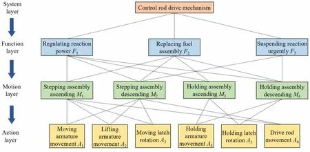
Fig. 3 (Color online) FMA structure decomposition diagram of CRDM
3 Flow field fusion simulation method based on model features
The motion of a CRDM in coolant is a fluid dynamics problem that can be solved using computational fluid dynamics. Because of the difference in computational principles between the IM and DMM for simulating objects moving in fluids,the simulation results of the same feature may differ between the two methods.A moving object is a collection of multiple features, which leads to inaccurate simulation results if each feature cannot be matched to a suitable method. Therefore, we required both methods to perform the simulation. We obtained the final results by extracting and fusing the simulation data applicable to each feature from the simulation results of both methods.
3.1 Contrast between IM and DMM
The IM fixes the moving object in the simulation and sets up the fluid inlet and outlet along the direction of motion in the computational domain. By replacing the original motion of the object with the flow of fluid relative to the object, the motion property of the object is transformed into the flow property of the fluid. After motion conversion, the iterative computation is reduced and the speed of convergence accelerated. Moreover, when the fluid reaches a steady flow state at the corresponding velocity, the results of each subsequent moment are the transient motion data of the object.Therefore,the accuracy of the simulation data is guaranteed.For the flow state,the simulation results of the IM around the moving object matched the real situation to a high degree. However, the state close to the inlet and outlet deviated because of the transition of motion.
The DMM sets the fluid to a static state at the beginning of the simulation and transfers motion information in the computational domain by squeezing the fluid mesh through the boundary of the object. The boundary is able to approximate the real situation after the motion parameters are set. Therefore, the fluid flow state obtained using the DMM is more accurate than that obtained using the IM[31]. Because the object is always in motion, a period of data must be processed, which leads to a large computational effort and prevents solving for a particular moment.Simulation errors at any moment in the period can affect subsequent calculations and even abort the simulation process. In the simulation process, the mesh near the boundary is involved in the motion and changes continuously,whereas the distant mesh remains constant because it does not meet the change requirements. This part of the mesh cannot participate in the calculation,resulting in low values for the fluid calculation. In addition, because the fluid in the computational domain is in a closed space, it circulates in the domain after the object starts moving.The motion at the next moment is disturbed by the circulating flow, causing fluctuations in the iterative process.
3.2 IM–DMM fusion simulation process
In this paper,fusion simulation method and a simulation process based on model features are proposed according to the aforementioned comparative analysis of the two simulation methods. First, we identified and classified the simulation units obtained by FMA decomposition as features and selected the simulation data to be used for each type of feature based on the applicability of the IM and DMM. Then, we improved the simulation models and operation settings of the IM and DMM in light of the selection results and performed the simulation analysis separately.Finally,we extracted the data required for each feature from the simulation results of both methods and fused the data in the order of feature merging to obtain the final simulation results. The specific operational process is illustrated in Fig. 4.The fusion simulation method matches the applicable simulation methods for the features in each category,thereby effectively solving the problem of the use of IM or DMM alone not being able to ensure simulation accuracy. Simultaneously, by organically combining the two simulation methods and focusing on the simulation data under specific features, we effectively improved the comprehensive application efficiency of the two methods.
· Step 1:Feature recognition of moving object simulation model We established the simulation model of the moving object by discretizing it into feature sets and identified the features that would affect the simulation results.Owing to their large number of features, the features were classified into fluid domain features and motion boundary features according to their attribution. We used the fluid domain features to describe the parameters of the flow field around the moving object and the motion boundary features to reflect the properties of the moving object. Among the two feature types, fluid domain spatial size and structural complexity were the features that strongly affected the simulation results;therefore,we chose them as indicators for the fusion of simulation methods.
· Step 2:Simulation data selection and method improvement based on features Each feature in the simulation model has a different applicability to IM and DMM. Therefore, before conducting the simulation, each feature for the simulation data of both methods should be selected and the simulation method be improved accordingly.

Fig. 4 (Color online) Fusion simulation process based on model features
The fluid domain constrains the flow range of the fluid,and its spatial size affects the fluid flow state.In a large spatial fluid domain, the DMM has difficulty in transferring motion information from the motion boundary to the mesh at the edge of the computational domain,which can cause biased results.The IM results should be used to ensure the accuracy of the flow field data. In addition, because of the distortion of the IM at the inlet and outlet of the computational domain, the determination of the fluid flow state should focus on the area surrounding the object. In the fluid domain of small spaces, the IM cannot obtain a sufficiently sized computational domain during the calculation, which leads to the fluid inlet and outlet being too close to the object,resulting in biased simulation data and disturbed fluid flow conditions. Therefore, the simulation results of the DMM should be used to obtain a realistic fluid flow. To alleviate the effects of excessive grid deformation and fluid circulation, the displacement of the boundary and squeezed flow should be reduced, which can be achieved by shortening the duration of mesh motion in a single simulation.
In our process of building the flow field simulation model, we simplified the structures that had less influence on the results.The retained structures affected the mesh quality of the computational domain depending on their complexity, resulting in a difference in the results produced by the two methods. For simple structures, the mesh size of the computational domain was divided moderately, and the mesh distribution in each region was uniform;therefore,both IM and DMM could converge quickly and smoothly to provide simulation results that are more accurate. For complex structures, the local meshes were small and densely distributed. Owing to the high sensitivity of the DMM to the quality of the mesh[32],small meshes are prone to errors in the updating process, resulting in a timeconsuming computation and a fluctuating iterative process. Therefore, IM results that do not require mesh-change operations should be used.
· Step 3: Simulation calculation and data processing We separately performed flow field simulations using the two improved methods and obtained the respective complete simulation data. We classified the data for each method according to the corresponding features,which were extracted and rejected based on the selection results in Step 2. The features were merged in their original order,and the corresponding simulation data were then fused to form the fused IM-DMM simulation results of the simulated object.
3.3 Applicability analysis of fusion simulation method
In addition to high-complexity structures, such as special-shaped latches and irregular armatures, the fluid domain space of a CRDM has different states, that is, a small fluid space in the motion region and a large fluid space in the nonmotion region, producing an unconventional flow field simulation. For a simulation object with diverse features, a single method cannot consider the characteristics of each feature,so obtaining accurate results is difficult.By formulating a suitable simulation scheme for each feature and fusing the data selected from multiple methods, the simulation results can benefit from the advantages of each method and more closely emulate the real situation. For general simulation objects, the diversity and complexity of their features are regular. Simulations using a single method can produce relatively reasonable results at the expense of accuracy;the simulation workload can be reduced by simultaneously omitting the data selection operation. However, if high-accuracy simulation results are required, the IM-DMM fusion simulation method based on model features is an effective method to solve such problems.
4 Application of fusion simulation method to CRDM
4.1 Preprocessing and feature recognition of CRDM simulation model
In this study, we used the CRDM considered by Deng et al. [33] as an example to verify the effectiveness of the proposed method. We established the fluid simulation model based on the physical model of the CRDM, and its local grid is shown in Fig. 5.We simplified the structure in the simulation model that had minor effect on the flow characteristics, with the following assumptions:
(1) The medium around the CRDM was a Newtonian fluid.
(2) The temperature of the fluid was constant (i.e., the adjustment of the reaction power by the CRDM did not affect the temperature of the fluid around it).
(3) The viscosity of the fluid did not change.
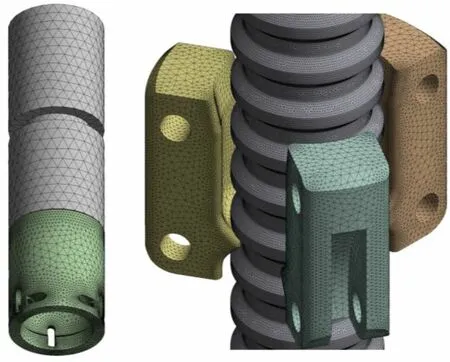
Fig. 5 (Color online) Local grid of simulation model
The radius of the computational domain was 200 mm,and the height was 1500 mm. The model parameters that we defined in Fluent are listed in Table 1. The boundary settings of the fluid calculation domain in the IM are presented in Fig. 6, and the corresponding boundary conditions are listed in Table 2.The basic fluid properties of the DMM were consistent with those of the IM; therefore, we only needed to set the parameters related to the dynamic mesh, as summarized in Table 3.
It is necessary to study the influence of mesh size on the solution before the simulation. We constrained the maximum mesh size to 50 mm and generated 11 groups of mesh schemes by dividing different minimum mesh sizes. Data for the mesh schemes are listed in Table 4, and the corresponding fluid resistance values are provided in Fig. 7.The hydraulic resistance changed remarkably in Case 1-4 but was stable in Case 4-11.This means that the number of grids was independent of the resistance after reaching 1.2 million. An increase in the number of grids improved the accuracy of the results,while increasing the computational cost. By combining the abovementioned factors, we determined the grid scheme of AS1-2-3-6with 1,891,738 grids. We obtained the grid scheme of AS2-3, which contained 289,422 grids, following the same method.
After establishing the CRDM simulation model, we identified the features of the model. The distance between the moving parts and the sealing shell in the CRDM is small, which limits the fluid space between the moving boundary and the wall. At the bottom of the CRDM, this area is connected to a large reactor space. Therefore, the simulation model had a large fluid domain, whereas the space for motion was small. In addition, parts of the latch,armature, and driving rod inside the CRDM have special structures,which increased the structural complexity of the simulation model. Therefore, the mesh size around these parts was much smaller than that outside the armature.

Table 1 Parameters of simulation model

Fig. 6 (Color online) Computational domain boundary

Table 4 The parameters of mesh schemes
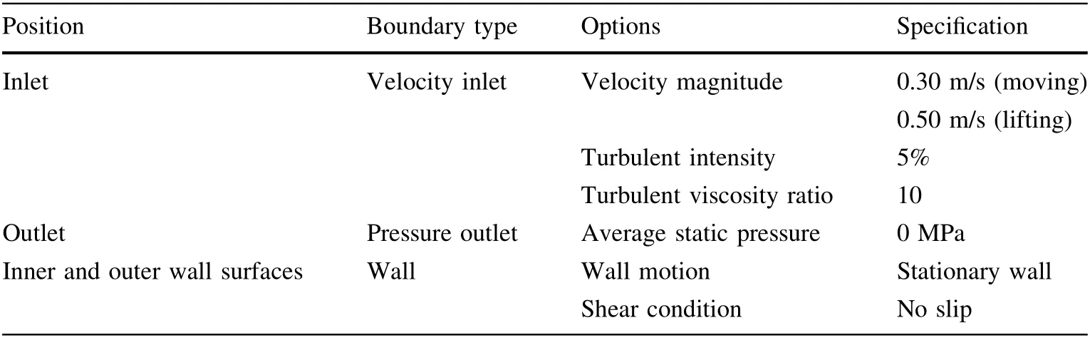
Table 2 Boundary condition setting of IM
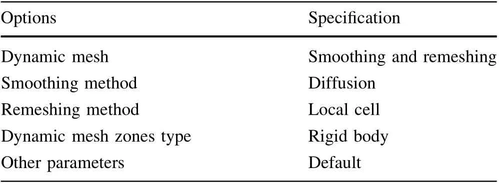
Table 3 Parameter setting of dynamic mesh
4.2 CRDM simulation data selection and method improvement based on features
The CRDM has a large nonmotion area,which increases the size of the entire calculation domain. Therefore, we adopted the resistance calculation value of the IM. Before the simulation, we appropriately extended the distance of the calculation domain from the inlet and outlet to the CRDM to reduce the influence of the distortion state on the simulation data.For the flow state,the result of the IM will be strongly affected,causing the motion area of the CRDM to be small; therefore, we used the flow state simulation results of the DMM. In addition, we appropriately increased the minimum mesh size within the deformation range to minimize the simulation failure caused by mesh update error.

Fig. 7 Grid sensitivity analysis
4.3 IM simulation results
US1-2-3-6accelerated in the upward movement, where the lifting armature reached a maximum speed of 0.5 m/s when it collided with the lifting pole. The simulation process and results for AS1-2-3-6at this time are shown in Fig. 8. As shown in Fig. 8b, the fluid resistance of US1-2-3-6was 3554.34 N. As shown in Fig. 8c, the fluid flowing in from the inlet was obstructed by the lifting armature and accumulated above it,causing the pressure in this area to increase and reach a maximum of 0.8 MPa.As the fluid flowed through the armature, the surrounding pressure gradually decreased and eventually dropped to zero at the outlet. The inner and outer surfaces of the lift armature and drive rod exhibited the same pressure. As shown in Fig. 8d, the fluid flowed along the central cavity of the drive rod, the gap between the drive rod and armature, and the space between the inner and outer wall surfaces after entering the computational domain.The fluid flow fluctuated as it passed through the drive rod owing to the undulating structure of the annular groove. The fluid flowing into the gap between the lifting armature and the driving rod increased instantly owing to the sudden reduction in the flow space, and the maximum flow speed was 1.62 m/s.When this part of the fluid continued to flow into the gap between the moving armature and drive rod,the flow space gradually increased and the flow velocity slowed. At the position of the latch and moving armature opening, the fluid velocity in each direction differed,forming a local pressure difference. The flow velocity was more balanced between the inner and outer walls. The velocity of the fluid close to the two sides of the wall was extremely low, and we observed a notable viscous phenomenon.

Fig. 8 (Color online) IM simulation process and results for AS1-2-3-6. a Residual curve; b Fluid resistance; c Pressure distribution; d Velocity vector and fluid streamline
The speed of US2-3increased in the upward movement,and the moving armature engaged with the lifting armature at a maximum speed of 0.3 m/s. The simulation process and results for AS2-3are shown in Fig. 9. As shown in Fig. 9b, the fluid resistance of US2-3was 436.77 N.Because the action pattern of AS2-3was similar to that of AS1-2-3-6, the changes in both flow field states were similar.As shown in Fig. 9c,the pressure at the top of the fluid calculation domain was as high as 0.15 MPa, and the pressure decreased from top to bottom, so the moving armature presented the same pressure state. According to Fig. 9d,the flow velocity of the fluid entering the cavity in the moving armature increased owing to spatial contraction.At the upper edge of the inner cavity,the flow path of the fluid was split into two, and the velocity at the separation point reached a maximum of 1.01 m/s.Uneven flow velocity and sticking also appeared at the latches and boundary walls, respectively.
4.4 DMM simulation results

Fig.9 (Color online)IM simulation process and results for AS2-3.a Residual curve;b Fluid resistance;c Pressure distribution;d Velocity vector and fluid streamline
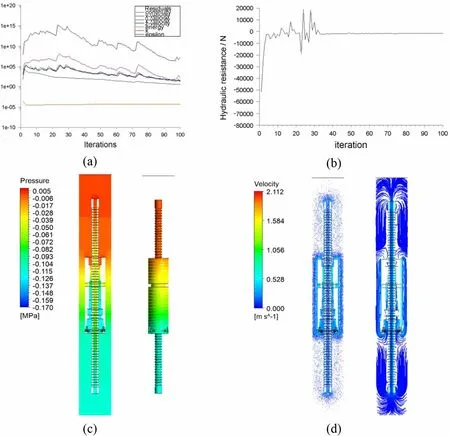
Fig. 10 (Color online) DMM simulation process and results for AS1-2-3-6. a Residual curve; b Fluid resistance; c Pressure distribution;d Velocity vector and fluid streamline
The DMM simulation process and results for AS1-2-3-6at a speed of 0.5 m/s are shown in Fig. 10. As shown in Fig. 10a, b, the dynamic mesh iteration process of AS1-2-3-6fluctuated considerably. At the beginning of the iterative process, the turbulent kinetic energy k in the residual curve oscillated upward, reaching a maximum in the 33rd iteration. During this period, the fluid in the computational domain was violently disturbed by the armature motion, and the calculation of fluid resistance showed large fluctuations. Subsequently, the value of k oscillated downward and converged gradually, and the fluid resistance stabilized quickly to 1472.13 N. As shown in Fig. 10c, the fluid above the armature was compressed,and the pressure rose during the upward movement of US1-2-3-6,whereas the fluid below the upper surface of the armature generated negative pressure because the fluid space increased. The maximum fluid pressure was 0.005 MPa, which occurred at the junction of the upper surface and inner cavity of the lift armature. Inside the moving armature, the inflowing fluid was obstructed and the velocity decreased, further reducing the pressure to a minimum of -0.17 MPa. The pressures of the inner and outer surfaces of the lift armature and drive rod were similar. As shown in Fig. 10d, the fluid in the computational domain generated a circular flow with the upward movement of US1-2-3-6. The fluid above the armature was squeezed upward, reached the top, and flowed back to the bottom of the domain along the outer wall surface, central cavity of the drive rod, and gap between the armature and drive rod. Owing to the small space in the inner cavity of the armature and the structural undulation of the drive rod annular groove, the flow velocity was higher in these two locations.A maximum velocity of 2.11 m/s occurred in the drive rod annular groove at the entrance of the inner armature cavity,while the fluid velocity near the outer wall surface was generally low.

Fig.11 DMM simulation process and results for AS2-3.a Residual curve;b Fluid resistance;c Pressure distribution;d Velocity vector and fluid streamline
The DMM simulation process and results of AS2-3at a speed of 0.3 m/s are shown in Fig. 11. As shown in Fig. 11a, b, the residual and resistance curves showed a small fluctuation at the fifth iteration. Subsequently, the residual value gradually decreased and stabilized, and the resistance value quickly converged to 205.76 N.As shown in Fig. 11c, the maximum pressure in the calculation domain was 0.019 MPa, which was located at the upper surface of the moving armature. The fluid below the moving armature showed a negative pressure, and the minimum pressure was -0.005 MPa at the lower surface of the moving armature. According to Fig. 11d, the fluid near the motion boundary moved at a substantially higher velocity than the fluid further away, and the fluid with a maximum velocity of 1.237 m/s was located on the upper surface of the armature.Near the latches and link holes,the negative pressure formed by the upward movement of US2-3created a large influx of fluid, creating a local highspeed region.
4.5 Data processing and accuracy verification of CRDM simulation results
In accordance with the selection of simulation data for different features,described in Sect. 4.3,we fused the fluid resistance from the IM and flow states from the DMM to form the final flow field simulation results of the key moving structural units in a CRDM. AS1-2-3-6received a fluid resistance of 3554.34 N, and the flow state during movement is shown in Fig. 10c, d. AS2-3received a fluid resistance of 436.77 N,and the flow state during movement is shown in Fig. 11c, d.
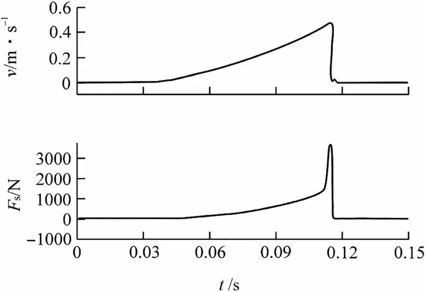
Fig.12 Movement speed and fluid resistance of CRDM in the lifting process [33]
At the beginning of the calculation, the state of the CRDM changed from static to moving, and the resistances obtained by the two simulation methods were remarkably larger. As the iterations progressed, the resistance gradually leveled. Deng et al. [33] reported the changes in movement speed and fluid resistance for the same CRDM during the lifting process. As shown in Fig. 12, before the collision, the speed of the CRDM was 0.5 m/s, and the fluid resistance at this time was about 3600 N. The experimental data were only 1.27% higher than the resistance of AS1-2-3-6in the IM after stabilization,whereas the resistance in DMM was much lower than that of the IM.This indicated that the resistance results of the IM were more accurate.The two methods exhibited similar trends in the pressure of the flow field around the CRDM. The pressure in the IM showed a stratified distribution with a maximum of 0.8 and 0.15 MPa for AS1-2-3-6and AS2-3,respectively,and a minimum of zero for both.The pressure distribution in the DMM spread along the direction of motion, with a maximum of 0.005 and 0.019 MPa for AS1-2-3-6and AS2-3and a minimum of -0.17 and -0.005 MPa, respectively. Because of the constant inflow of fluid from the inlet,the maximum pressure in the IM was high.In contrast,the amount of fluid above CRDM is the same as the actual situation in DMM, so its maximum pressure was more accurate. In addition, negative pressure is generated behind an object along the direction of motion as it moves in a fluid [18]. The results of the DMM (Figs. 10c and 11c) reflected the negative pressure region at the bottom of the CRDM, whereas the minimum pressure in the IM results was always zero. In realistic motion,the upward movement of the CRDM increases the velocity of the local fluid and circulates the fluid within the computational domain. This phenomenon was accurately represented by the results of the DMM(Figs. 10d and11d),whereas the fluid flow direction of the IM was always unidirectional from the inlet to the outlet of the computational domain (Figs. 8d and 9d). In summary, the fused simulation method integrates the fluid resistance from the IM and the flow state from the DMM and eliminates distortions in the data caused by the calculation principle of each method so that the accuracy of the final simulation results is high.
5 Conclusion
To perform an efficient and accurate flow field simulation of a CRDM,in this study,we constructed a fused flow field simulation method based on model features. First, we decomposed a CRDM into several meta-action units by FMA analysis, and identified the lifting meta-action set AS1-2-3-6and the moving meta-action set AS2-3as simulation nodes according to the linkage relationship between the meta-actions and their influence on the flow field.Then,we established a fused feature-based IM-DMM simulation process and characterized the CRDM by a large fluid domain, small motion space, and complex part structure.After comparing the applicability of different simulation methods to the features of the simulation model, we selected the fluid resistance of the IM and flow state of the DMM. Based on the selection result, we extended the distance between the inlet, outlet, and CRDM of the calculation domain in the IM and increased the minimum mesh size in the DMM to within the allowed range of deformation. Finally, we extracted the required data from the simulation results for each feature and obtained the results by fusing the simulation data in the order of the features.
Authors contribution All authors contributed to the study conception and design. Material preparation, data collection and analysis were performed by Si-Tong Ling,Wen-Qiang Li,Chuan-Xiao Li and Hai Xiang. The first draft of the manuscript was written by Si-Tong Ling, and all authors commented on previous versions of the manuscript. All authors read and approved the final manuscript.
Declarations
Conflict of interest The authors declare that they have no known competing financial interests or personal relationships that could have influenced the work reported in this paper.
杂志排行

Nuclear Science and Techniques的其它文章
- Design and tests of the prototype a beam monitor of the CSR external target experiment
- Development of a wide-range and fast-response digitizing pulse signal acquisition and processing system for neutron flux monitoring on EAST
- On the viability of wearing evaluation by Thin Layer Activation in the presence of non-occupationally exposed individuals
- Enhancement in optical absorption of CsI(Na)
- Research on tune feedback of the Hefei Light Source II based on machine learning
- Development of a subchannel code for blockage accidents of LMFRs based on the 3D fuel rod model