On the viability of wearing evaluation by Thin Layer Activation in the presence of non-occupationally exposed individuals
2022-05-12MicheldeAlmeidaFrancJulioCezarSuitaPauloFernandoFerreiraFrutuosoMeloCelsoMarceloFranklinLapa
Michel de Almeida Franc¸a· Julio Cezar Suita · Paulo Fernando Ferreira Frutuoso e Melo ·Celso Marcelo Franklin Lapa
Abstract Thin Layer Activation is a nuclear technique that has key advantages over other wear measuring techniques for mechanical systems, especially for in site experiments on equipment important to safety in nuclear plants. Still,it incurs radioactive dose and, thus, must be proved radiologically safe before use, otherwise, the utilization of this technique may be hindered inviable. Proving said technique is safe previous to any operational/monetary cost is key,providing a methodology for this early assertion is the main contribution of this work-here, only non-occupationally exposed individuals are considered. This work offers a methodology,through a case study,to ascertain the Thin Layer Activation parameters to obtain safe levels of radioactive dose while maintaining statistically reliable results. This methodology consists of using simulations,through the Monte Carlo Method, to obtain the floors and ceilings for the previously mentioned activation parameters based on operation and work conditions on site.
Keywords Thin Layer Activation · Safety evaluation ·Simulation · Equipment wearing
1 Introduction
Currently, around 300 nuclear power plants (NPPs)across the globe are over 30 years old [1], most of them have gone already, or will go, through the useful life extension process, which is a key part of maintaining nuclear power competitive [2]. Such a process is complex and requires the assertion of a plethora of parameters,most of them related to safety standards [3]. Thus, these parameters must be acquired with high levels of precision and reliability. However, one complicating factor in the assertion of said parameters is the fact that these plants are operating while the inspections for life extension happen,thus disassembling or ceasing their operation goes against safety and reliability standards.
One of these parameters is wear, a common phenomenon to any material. And, more specific to this work,wear is related to friction, which is present, in a relevant way, in many important to safety systems, such as emergency water pumps and generators [4]. This type of wear,occurs mostly due to moving parts and chemical factors[5].Another aspect prominent in the life-extension scenario is obsolescence, where systems are replaced by newer models, or entirely new combinations, creating systems that must be monitored through their life.
The analysis of wear can be done through a few methods,some of non-nuclear nature,others nuclear[6].On the non-nuclear side, a few methods stand out, such as precision scale and 3D measuring machines. These methods,however, fall short when they meet the previously mentioned need to interfere with the systems as little as possible, as they require multiple disassemblies to acquire data over a period of time. For the nuclear ones, two common measuring methods are activated material insertion and neutron activation:the former has the drawback of changing the chemical and mechanical properties of systems so important to operation; the latter may not be used in site, as it requires the entire piece to be homogeneously activated by a neutron source, giving off high levels of radioactive dose to anyone in the vicinity [7]. Still on the nuclear side, one wear measurement technique that addresses both challenges, requiring only one interaction with the system parts (possibly on its first assembly),allowing in site long and periodic measurements,while still giving off low levels of radioactive dose, is the thin layer activation (TLA) [8].
This technique consists of activating a small region on the surface of a system part with a charged particle beam.This activation is homogeneous up to a certain depth,thus,when material is removed from said surface,the registered activity-using an adequate gamma detection systemwill be proportional to the depth of wear.This technique is discussed in depth ahead.
While TLA has its advantages over other techniques,as discussed previously, its competitiveness can still be improved through a few factors.Since its main downside is being a source of radioactivity,asserting the effective dose to any personnel involved previous to any interaction with the plant operation and for a low time/resource cost will greatly improve its applicability.Thus,this article provides a methodology for such assertion at low costs using Monte Carlo simulations.
Said assertion aims to determine which activation/experiment parameters would result in good statistics while still being safe, regarding radiation dose, for in site experiments, especially for non-occupationally exposed individuals(NOEI)-here,the choice for using only NOEI as the parameter was made because both occupationally exposed individuals(OEI)and NOEI will be present at the vicinity of the analyzed equipment and, since NOEI have far lower legal safe levels for radiation dose, they will always represent the lowest ceiling for maximum dose levels. As the goal is to determine activation parameters prior to the activation itself and any interaction with the system that will be activated and analyzed, if possible,simulation is the perfect approach to this methodology. In this instance,the Monte Carlo N-Particle(MCNP)code[9]will be used (for availability reasons), also discussed in depth ahead. Brazilian radiological standards will be considered, especially the ceiling for yearly effective dose for NOEI, which is 1 mSv [10]. As for comparable studies,while there are studies related to radiation dose and Thin Layer Activation[11],they often do not address NOEI and those that do, do it post application. Thus, there is a necessity for a methodology to predict how safe such experiments will be.
This paper is organized as follows: Section 2 contains the pertinent information on techniques and materials used;Section 3 describes the methodology used,step-by-step,to achieve the goals previously mentioned;Section 4 presents the results obtained and their discussion; Section 5 contains the future prospections for this work; Section 6 displays the conclusions and recommendations.
2 Fundamentals and materials
This section describes the main techniques, programs and materials used in this work,as they might be specific to this case, but can also be pointed out as a general methodology for this type of assertion.
2.1 Thin Layer Activation
Thin Layer Activation is a technique mainly used for wear analysis. It allows low activation levels as it only activates a very small portion,around 0.7mm diameter and a depth that goes from 50 μm(using the standard activation method [8]) to 300 μm, the latter being achieved by using an activation technique developed in previous work [12].This depth, coupled with the variety of options for the activation beam, also brings a range of experiment durations, for example: on an iron-based alloy, there are two main possibilities of charged particles to be used, Proton and Deuteron, the first gives the following reactionnatFe(p,x)56Co,the laternatFe(d,x)57Co,with 77 and 271 days of half life,respectively[13].This range of half lives,in turn, allows shorter and longer experiments, especially for those systems that must be monitored for longer periods, even allowing maintenance and cost savings, with higher and lower radiation levels for different scenarios of operation for the target of wear analysis, and deeper activation for systems that can sustain more wear while maintaining their reliability.
The most important part of this technique is that this activation must be homogeneous up to that certain depth,this allows one to linearly correlate the decrease/increase in detected radioactivity on the activated piece surface with removed material from the said surface (through wear).This linear correlation is achieved through the analysis of the stopping power of a charged particle and a given material (for example, deuteron on Steel 1020), this analysis returns the ideal energy at which the charged particle will hit the surface to obtain the desired homogeneous activation up to a certain depth.Figure 1 shows an example of such an arrangement, using deuteron on Steel 1010,whose ideal energy is 7.2 MeV and creates a homogeneous depth of around 15 μm through the reactionnatFe(d,x)57Co.

Fig. 1 Example activation profile for deuteron on Steel 1010 [8]
On the detection system,it is important to note that there are two different methods: the thin layer differential method (TLM), where, basically, the detection system is pointed at the activated source and registers the decrease in its activity and concentration measuring method (CMM)[14], where the detection system is pointed at an accumulation point for the removed material; this method registers the increase in activity.
2.2 TLA2 tool
This tool is used multiple times throughout this work.It,in short, makes the stopping power and cross-section calculations for all reactions of interest to wear analysis using Thin Layer Activation [8]. The input consists of: the material (in our case, an alloy) that will be activated; the charged particle used;activation beam parameters, such as current,irradiation angle and time of exposure and cooling period.
It then returns the results with a profile of activation,such as seen in Fig. 1. The two most important data, from this tool, for this work are: total activity for the source,including the entire activated area, not only the homogeneous part(marked with the blue line)and specific activity,which is the activation per micrometer throughout the homogeneous area. Their uses will be discussed ahead.
2.3 Monte Carlo N-particle code
This program/ambient is used to simulate nucl ear reactions [15]. In this work, for availability reasons, the MCNP-X version is used. It consists of using an input file that contains the following informations:
· Geometry-materials, their shapes, densities and positions;
· Source-which particle is emitted, from which cell, on which energy and directions;
· Output mode-which type of result is required, effective dose, pulse height distribution and so on;
· Number of Stories-This defines the number of iterations done by the MCNP-X, and the final precision for the simulations.
In this work, pulse height distribution (through the F8 function) and effective dose results (using the F5* function)are used.For effective dose,there are also the de and df cards [16], which act as a weight function that turns the results from F5 (particle flux on a punctual detector) into effective dose. The values of these cards, as used for this work, are seen in Table 1. This function and its precision were tested on a previous work [17].
It is worth noting that all results from MCNP-X must be multiplied by the number of emitted particles, or disintegrations and the probability of each gamma peak, for example.This is necessary because all results from MCNPX are composed of ‘‘efficiencies’’, as in the fraction of 846 keV gammas emitted by the source that will actually be detected by the detection system, or the effective dose,in pSv, per emitted gamma by the source. Those efficiencies, from now on, will be referred to as counts/emission and pSv/emission, respectively.
3 Methodology
The flowchart presented in Fig. 2 contains the methodology used in this work in a concise manner, while the following sections and paragraphs go into detail on each step and decision made to apply our methodology to a specific system, which is analogous to a system important to safety. Said methodology has the main goal of keeping radiation levels under safety limits while still delivering good statistics.
3.1 Choosing analyzed system and its environment
The first step is to choose a system to be analyzed. The chosen system must:

Table 1 Values for de and df and their respective energies

Fig. 2 Methodology flowchart
· Have an analogous operation and design as those important to safety in nuclear power plants;
· Generate wear due to removal of material from its surface;
· Have available schematics, or access to them for measurements, to allow precise simulations;
· Present a varied level of complexity and materials.
Other choices made in this step reflect which experiment would be requested by a contractor, or under what conditions the analyzed system would be operated. The main aspects here are: how much wear can it generate and sustain;how long should the experiment last,or how long are we to analyze the wear on it and how close to the system are the personnel and how long they stay at that distance.
These, in turn, will affect the choices of which method(as pointed out) and which charged particle (proton or deuteron, for example) will be used to activate the target and how close the personnel will remain to the source and for how long and, lastly, how active the source is.
3.2 Design of analyzed system in MCNP-X
In this step, the chosen system is designed, from the previous step,with the help of MCNP-X.This process may use a range of precisions, however, two aspects must be made as accurate as possible: material compositions and densities, as they heavily influence the absorption of gamma rays and; any geometry that will be between the activated source and any personnel in its vicinity.
As for the geometries of components and materials that will not stay between the source and personnel,they can be streamlined and simplified for faster simulations and, thus,achieve our goal of using a faster and more reliable method to ascertain the TLA applicability for a given scenario.
3.3 Dose simulation
As the system part that will be analyzed is composed of an alloy and will be activated through a charged particle beam, several unstable isotopes will be created in that small region. The TLA2 Tool is used to determine what is the resulting activation and, from that, one obtains the list of emission lines, their emission rates and probabilities.
Note that it is a common practice to let the part cool for about 7 days before the experiment;this allows the isotopes that have shorter half lives to decay and be less of an interference.
After this early analysis of which gamma lines will be present in the source,some of those lines can be merged as they have small emission probabilities. These mergings help to streamline the simulations, as each line must be simulated separately. A round of quick tests can be performed to prove that such mergings will not affect the results in a significant manner.
The dose simulation in MCNP-X is done by using the F5 function coupled with the de and df cards. These cards act as weight functions, which take the detection efficiency vector given by the F5 function and turn it into a dose efficiency, as pSv/emissions. ‘‘Emissions’’ in this case is given by the source activity, for example, if a source has 100,000 disintegrations per hour, then, multiplying the result from the F5 plus de and df cards by 100,000 will return the effective pSv/h dose for this scenario.The source activity is either a given value based on an existing activation or is an arbitrary value decided in a previous step,Sect. 2.1.
As the source activity is introduced after simulation,the variations that must be done in this step are made up by distances from source to detector,the use of shielding,such as lead sheets and which isotopes are present in the source.Results obtained here are kept for comparisons with those of the next step.
3.4 Detection geometry simulation
While the dose simulation will tell whether the experiments are safe, these latter still have to provide useful and reliable results. In this regard, the approach used in this work is to simulate a reasonable geometry for detection systems in MCNP-X and, using the F8 function, obtain detection efficiencies. Once again, these results must be multiplied by the number of disintegrations from the source to return the final result as counts per second, or total counts for an experiment of a given duration.
For this work, two different durations were considered:30 min and 3 h long experiments. These depict shorter experiments for interfering with the workplace as minimum as possible is a necessity and longer experiments, so that procedures do not affect the work place meaningfully.
3.5 Activation level determination
Activation levels are determined through the combination of: particle type; current of the beam and exposure time.The TLA2 tool handles these calculations and returns the effective source activity.
Thus,using said tool,it is possible to arbitrarily obtain a range of activations,which have two sets of important data:total activity, including all isotopes (merged in fewer emission lines,as described previously),which is used with effective dose efficiencies; and, main isotope activity(846 keV for56Co, for example), which is used for counts per second and total counts calculations.
To assert the minimum activation level, the statistical uncertainty is the most important aspect. This work aims for 1% uncertainty-which corresponds to the most common goal for industry level experiments-, which correlates to 10,000 total counts-disregarding background.The total counts are obtained by multiplying the detection efficiency obtained in the previous step by the number of disintegrations/emissions from the source, on a given period of the experiment (30 min and 3 h, as discussed previously).
After the minimum activation level being set, the maximum activation is set through the analysis of effective dose. This requires the combination of results from simulations and arbitrary levels of activation,which then results in pSv/h, described in depth at Sect. 3.3. Finally, this is multiplied by the number of hours a person is supposed to remain at the simulated distance and position.The effective dose obtained here is then compared to the target maximum values, determined by radiological laws on its workplace.
Here, an addendum should be included: while this article was limited to a specific scenario of combining TLA technique, important to safety equipment and NOEI, the methodology presented here can be extended to other scenarios. As discussed previously, this technique can be applied for longer periods of time, even years, if the activation is increased, such increase would also imply an increase in radiological dose and determining the activation/dose levels ratio through the methodology presented here greatly improves the applicability of wear analysis through TLA while keeping its other advantages over the competitive techniques.
4 Results
The results presented ahead represent a set of possibilities for the experiment explored in this work and show what are the viable options for it.
4.1 Choosing analyzed system and its environment
The chosen system is the TE 92-6-5 by Phoenix Tribology Ltd. [18]. This system addresses all the prerequisites: generates wear through rotation and friction; it is, in fact, a tribometer, which is meant to generate wear at a controlled manner; it is available to us at a partner laboratory (Laborato´rio de Tribologia e Metrologia Dimensional COPPE/UFRJ); has detailed schematics available;and, allows the use of a vast variety of alloys. Also, one major beneficial aspect of this choice is that, as it is a tribometer, it offers counterproof of wear analysis for our technique in future works. This tribometer is shown in Fig. 3,while its main part’s schematics is shown in Fig. 4.
For the remaining aspects chosen here, the activation technique was locked to the regular type and the increased depth activation technique will not be used, as this tribometer is suited for fine wear rather than longer experiments or softer materials.On the material side,for reasons of availability,Steel 1010 will be used for the analysis,it is iron-based;a choice for a proton was also made. Thus, the reaction used isnatFe(p,x)56Co, with an analyzable emission life from the56Co at 846 keV.
The non-occupationally exposed individuals working conditions in site are composed of combinations of the following possibilities:distance source-personnel of 30 cm or 100 cm; and permanence, at said distances, for 5 h and 40 h per week, and a working year of 48 weeks. Those 4 combined scenarios will be considered in the effective dose evaluations.
4.2 Design of analyzed system in MCNP-X
The design aimed to be more detailed on the areas between the source and personnel/detectors. The other areas were either less detailed or simply not designed in the MCNP-X ambient,for example,the design stopped around 100 mm above the source and 50 mm under. Figure 5 shows the TE 92-6-5 design inside the MCNP-X ambient.
The colors here represent the material of each cell, for this case:pink=air;yellow=industrial aluminum;green=cast iron; light blue = generic mineral lubricant oil; red =steel 1010; and, dark blue = the source, which is made up of the same 1010 steel, and is activated and has traces of different isotopes (discussed further ahead) and56Co.
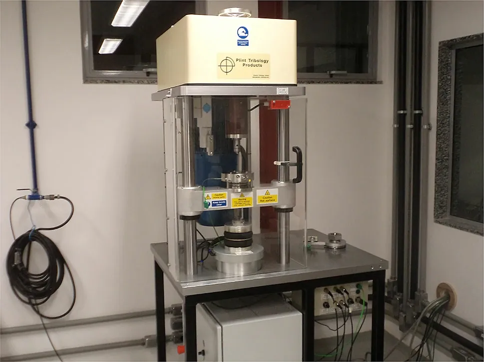
Fig. 3 (Color online) TE 92-6-5 in site
This system does not support indirect measures(through a filter,for example),thus,only one detector was simulated here. This detector, as previously discussed, may be used with a few configurations, including size and positioning.However, for the purpose of display, Fig. 6 shows one of those options, with a NaITl detector and its components.
Table 2 contains the materials used in said models. The colors from Figs.5 and 6 were used for a better assessment of these informations.
4.3 Dose simulation
For 1010 steel hit by a proton beam, the resulting activation profile after a seven day cooling period can be seen in Fig. 7.
The dose efficiencies, for 30 cm and 100 cm positions for each emission line are listed in Table 3.Since how long will be the activation, and, thus, what are the total and specific activities on the source is still arbitrary at this step and will be discussed ahead, here, these efficiencies are represented in pSv/emissions and will be converted to pSv/h and total mSv on a later step.
It is important to note,from Fig. 7,how disproportionate the56Co isotope is, compared to all byproduct isotopes.This allows for a dose analysis based only on the emission lines from56Co[13].These,were merged in 10 lines.This process was tested and returned only a 2% increase as to the effective dose. This process significantly reduced the simulation time. The resulting 10 emission lines are also listed in Table 3.
4.4 Detection geometry simulation
For the TE 92-6-5 tribometer, a 10 cm system-detector distance is reasonable, it should also be safe from movements and heat for the detector in most scenarios. Thus,this was the only distance used.The detector used here is a 2×2′′NaITl detector, enclosed in the lead but uncollimated. This choice is based on the fact that using a less efficient detector would increase the effective dose, as it would require a more active source for the same statistics.This detector is also widely available and rather simple to use in site, as it does not require refrigeration [20].
For this scenario, the efficiency obtained was 1.75×10³counts/emissions. This value will also be converted in the next step.
4.5 Activation level determination
Here, the efficiencies are taken and multiplied by arbitrary values of activation.There is a separate value for total activity, including the entire activated source, and a specific activity, which comprises only 1 μm from the surface of the source. Both are calculated by the TLA2tool. Through these, we can ascertain the minimum activation levels for our experiments to return the desired precision. For 30 min long experiments: total source activity is at 750 kBq and specific activity at 3.21 kBq/μm.
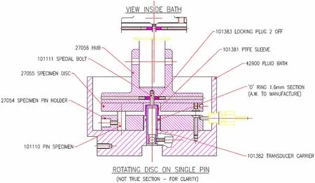
Fig. 4 TE 92-6-5 schematics

Fig.5 (Color online)TE 92-6-5 design inside the MCNP-X ambient,using Vised program for visualization [19]
The effective dose values set the maximum activation level for this experiment to comply with the radiological regulations. Here, only two scenarios are shown: one considering a close source-personnel distance, but with a shorter-but still realistic-exposure time and the other,with a reasonable distance, possibly setting hazard markings on the ground,but considering that personnel will be allowed to stay at that distance for all of their working hours,which is the worst-case scenario.Observing these,it is possible to infer the following maximum source activation:

Fig. 6 (Color online) TE 92-6-5 and Detector design inside the MCNP-X ambient, using Vised program for visualization
· At 30 cm distance, personnel-source, for a period of 5 h/week, the maximum total source activity is at 900 kBq and specific activity at 3.80 kBq/μm. This scenario returns a yearly effective dose of 0.97 mSv,this is just under the maximum threshold of 1 mSv/year set by regulatory agencies;
· At 100 cm distance, personnel-source, for a period of 40 h/week, the values are 1350 kBq for total activity and 5.78 kBq/μm. This scenario also returns a yearly effective dose of 0.97 mSv.
After obtaining the floor and the ceiling for our activation levels, the next procedure would be to activate the source considering these limits. However, this work has achieved its goal here:determining that this experiment is safe to beperformed in site, even in the presence of non-occupationally exposed individuals. Meanwhile, also establishing a safe, fast, reliable and almost costless way to assert radiological safety for Thin Layer Activation experiments.
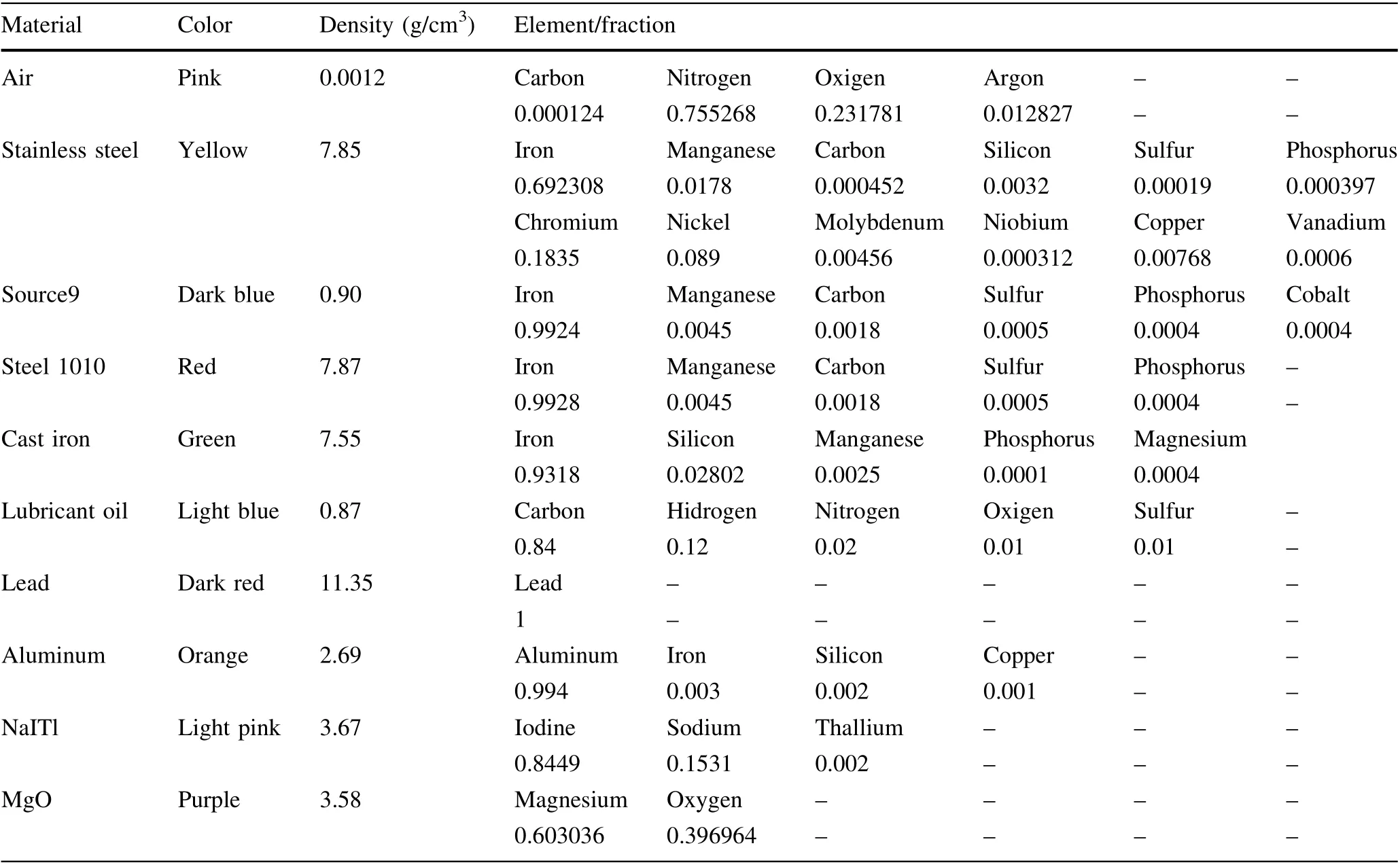
Table 2 Materials used on the simulations

Fig. 7 Activation profile for proton beam on steel 1010

Table 3 Dose efficiencies
5 Discussion
With the results in hand, we can attest that this methodology is effective at defining the activation parameters for safe and statistically reliable Thin Layer Activation experiments on physical wear. However, some other improvements and additions can be made to what was achieved in this work, for example: doing the activation and experiments to attest the obtained data, while the parameters used in MCNP-X are already largely tested and seen as a reliable method to obtain such data,testing it with experiments on our geometry and parameters is always a great addition, said experiments will be performed in the near future.Another addition that could be done to the data and methodology presented here is a study relating the wear measurement to failure rates and impacts on equipment management,with a broader discussion on reliability using known statistical methods, based on the findings obtained through this methodology.
6 Conclusion
The methodology presented here uses the MCNP-X ambient to simulate a Thin Layer Experiment before the activation is performed. And, while doing so, analyzes whether it is safe to conduct such an experiment in site,while non-occupationally exposed individuals are in the same area. This methodology will provide the activation parameters in a fast and safe manner, while interfering as little as possible with the wear. Also, for future prospections we recommend the development of an FMECA(Failure, Mode, Effects, and Criticality Analysis) in order to search for potential TE 92-6-5 failure modes and how they affect wear generation. In this case, it is possible to rank the failure modes by means of a criticality index.There are different ways to define and use this criticality index, for example, MIL-STD [21], Guimara˜es and Lapa[22], Garcia et al. [23]. Uncertainties in these definitions may be tackled by means of fuzzy logic, as in these two latter references.Also,it would be advisable to discuss the use of fuzzy rule interpretation Baranyi et al. [24] due to the possibility of sparse rule bases and complexity reduction as related to the identified failure modes.
杂志排行

Nuclear Science and Techniques的其它文章
- Design and tests of the prototype a beam monitor of the CSR external target experiment
- Development of a wide-range and fast-response digitizing pulse signal acquisition and processing system for neutron flux monitoring on EAST
- Enhancement in optical absorption of CsI(Na)
- Research on tune feedback of the Hefei Light Source II based on machine learning
- Development of a subchannel code for blockage accidents of LMFRs based on the 3D fuel rod model
- Robust restoration of low-dose cerebral perfusion CT images using NCS-Unet