An optimized numerical method to pre-researching the performance of solid-phase oxygen control in a non-isothermal lead–bismuth eutectic loop
2022-05-12XiaoBoLiRuiXianLiangYiFengWangHuiPingZhuFangLiuYangLiuCongLiHaoWuFengLeiNiu
Xiao-Bo Li · Rui-Xian Liang · Yi-Feng Wang · Hui-Ping Zhu · Fang Liu ·Yang Liu · Cong Li · Hao Wu · Feng-Lei Niu
Abstract In the present work, a new transient calculation method for parameters that can be used to evaluate the ability of oxygen control in a non-isothermal lead-bismuth eutectic (LBE) loop with solid-phase oxygen control was proposed. It incorporates the dissolution process of PbO particles and the oxygen mass transfer process, and an optimized method was used for finding out the optimized oxygen mass transfer coefficient.In numerical terms,three mass transfer models were simultaneously applied, and comparisons of calculated and experimental results from the CRAFT loop indicated that the optimized calculation method and these new oxygen mass transfer models were correct and applicable to other LBE loops. Through this calculation method,we aimed to optimize prediction of the distribution of oxygen and iron concentrations, time taken to establish the steady state of oxygen, and maximum dissolution/precipitation rates of corrosion products and corrosion depth across the entire LBE loop. We hope that this work will provide a potential reference for designing a more intelligent oxygen control system in the future.
Keywords LBE · Solid-phase oxygen control · Operating domain · Operating model · Corrosion depth ·Dissolution/precipitation
1 Introduction
Lead-bismuth eutectic (LBE) is globally regarded as a candidate coolant for Generation IV fast reactors [1, 2]because of its favorable thermophysical properties.Despite many promising properties of LBE, its compatibility issue with structural materials remains a matter of concern.Therefore, corrosion (mainly including dissolution and oxidation)occurs in heavy liquid metals(HLMs),which is one of the critical obstacles to the widespread use of LBE as a nuclear coolant [3-6] and depends on the oxygen concentration in the coolant [7].
According to the Ellingham diagram, oxygen activity control is a widely used method to mitigate corrosion,which involves the formation of protective oxide scales on steel without oxidizing the HLMs [7]. Due to the consumption of oxygen by the oxidation of the material,oxygen must be supplied continuously and precisely to the LBE loop during operation. Gas-phase oxygen control techniques have been successfully applied to control the oxygen concentration in LBE systems. However, the main drawbacks are the risks of slag formation and possible release of radioactive isotopes because of overpressure. A solid-phase oxygen control by a solid PbO mass exchanger(MX)can fully avoid these disadvantages,and by adjusting the LBE flow rate through the MX and its temperature,the supply rate of oxygen to LBE can be controlled [8].Experiments on solid-phase oxygen control technology have been carried out internationally [9-13] and have included MEXICO and CRAFT loops at the Belgian Nuclear Research Institute (SCK·CEN), SM-2 and TT-2M loops at the Russian Institute of Physics and Dynamics(IPPE),and the DELTA loop, a large-scale test loop at the Los Alamos National Laboratory(LANL)that can be used for LBE solid-phase oxygen concentration control technology research(a summary is displayed in Table 1).Solidphase oxygen control techniques easily regulate oxygen concentration in an LBE system; however, few studies are available regarding such solid-phase oxygen control techniques,and there is a lack of experience in their design and operation. Moreover, the oxide corrosion rate is mostly dependent on the oxygen concentration and thermohydraulics of the fluid, especially the operating temperature and flow rate of liquid metal [7, 14, 15]. Therefore, to develop an effective design, especially to determine accurate boundary conditions for long-term operation in an equilibrium state,it is necessary to extensively analyze the factors that affect the oxygen concentration and corrosion depth in the loop.In the present study,a simulation method was used due to the amount of available pre-experimental research.
In past decades, the simulation method was considered an effective method for simulating multidimensional and complicated behaviors in LBE-type fast reactors [16-18].Modeling of metal oxidation and dissolution/precipitation in liquid LBE has previously been conducted [19-23]. It should be noted that previous corrosion modeling generally assumed a constant oxygen concentration distribution in the loop, which is definitely not the case when using a solid-phase oxygen source, and the corrosion product concentration in bulk LBE flow was generally simplified as a constant. Such hypothetical simplification eliminates the possible influence of distribution in-homogeneity of corrosion products on the dissolution/precipitation equilibrium and vice versa. To pre-research the performance of solidphase oxygen control in a non-isothermal LBE loop, the transient simulation of oxygen concentration distribution in the loop needs to consider both the consumption of oxygen caused by corrosion and the oxygen provided by oxygen source. In addition, the formation and stripping process of the oxide layer is too complicated. It is difficult to characterize the total oxygen consumption rate through the present models [19-23]. Therefore, the present work, by considering the conservation of oxygen concentration in the entire system, aimed to tailor an optimized corrosion model to our non-isothermal LBE loop with a solid-phase oxygen control system. Moreover, this method combined the dissolution model of solid-phase PbO particles with an overall oxygen flux model based on the mass transfer coefficient in the LBE loop. Subsequently, it was possible to establish and transiently solve the conservation equation of oxygen and iron concentrations in the LBE loop. The oxidation process was mass transfer controlled, and the mass transfer coefficient of oxygen was calculated in the same way as for iron[24].Finally,the time to establish the steady state of oxygen, oxygen concentration, maximum dissolution/precipitation, and corrosion depth in the equilibrium state and with different causes were calculated.Additionally,the ability to control oxygen in the LBE loop is discussed based on these simulation results. Meanwhile,a safety operating domain in our non-isothermal LBE loop was determined.
2 Experiments and optimized simulation method
2.1 Experimental setup
A 3D non-isothermal LBE loop built is shown schematically in Fig. 1. The MX, in which PbO particles were stored, was installed onto the solid-phase oxygen control bypass module. By tuning the mass flow rate and temperature within the bypass module, the amount of oxygen released from PbO MX to liquid LBE became adjustable.As presented in Fig. 1c,d,an electric valve was installed onto the solid-phase oxygen control bypass, and its operating model can be changed with the operating state of the valve. When the mass flow rate in the main loop remained constant, the flow rate through the MX was minimal when the valve was fully open,while the MX took the maximum flow rate that was equal to that of the main loop when the valve was closed. A venture design was taken at the outlet of the oxygen control bypass that increases the lower limit of the flow rate through the MX under operating model 2.
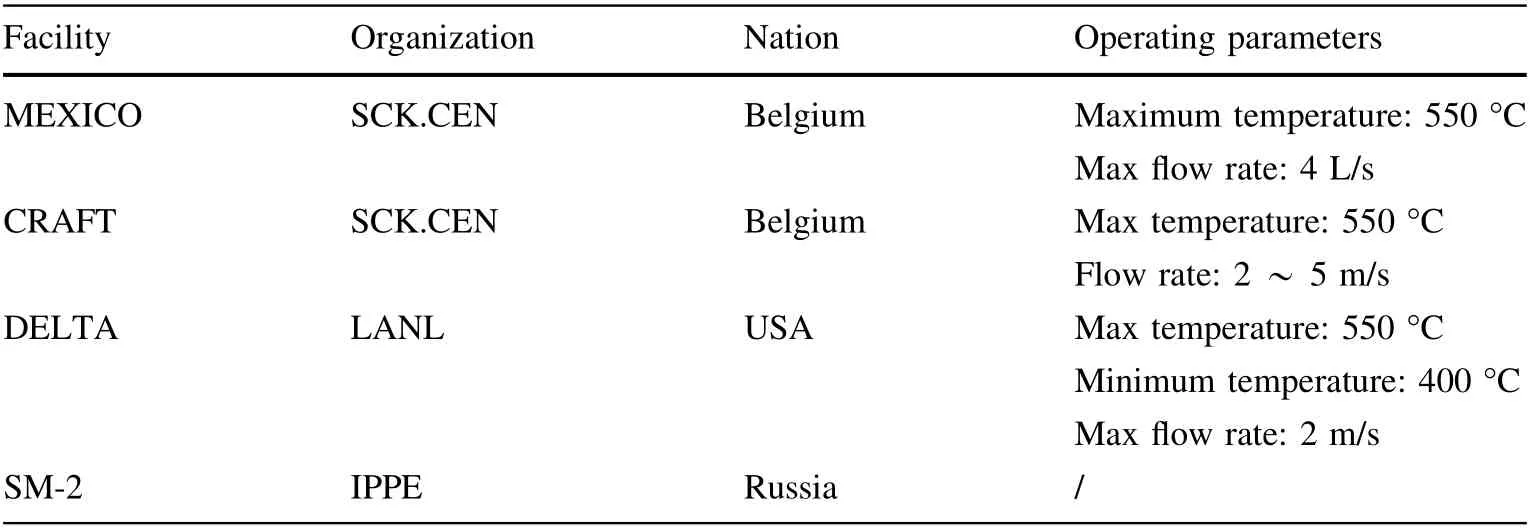
Table 1 Loops with solidphase oxygen control and their operating parameters
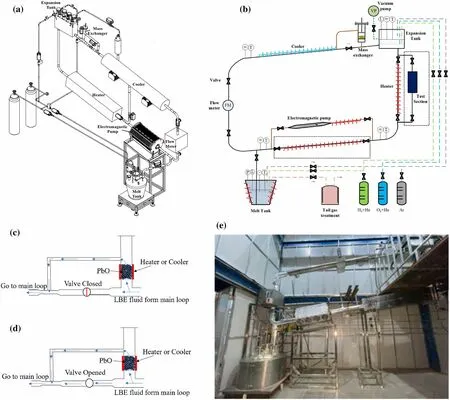
Fig. 1 (Color online) LBE loop in this project: a three-dimensional view of the loop design, b two-dimensional view of the loop design,c operating model 1, d operating model 2, and e overall appearance of the loop
2.2 Mass transfer model
The mass transfer process of oxygen content dissolved in the liquid LBE is illustrated in Fig. 2a, and a reaction layer at the solid-liquid interface was assumed to be established here (Fig. 2b). The contribution from LBE and iron ions in LBE fluid to oxygen consumption was small under the oxygen control environment. Therefore, the fluctuation of the oxygen concentration in the ith control volume might be associated with the initial dissolved oxygen in the control volume, oxygen flux out of the control volume, oxygen flux from the solid oxygen source located in the oxygen system, and oxygen flux into the reaction layer. Between the latter two factors, the level of dissolved oxygen might stem from the dissolution of both PbO particles and other metal oxides at a high temperature.
The oxygen concentration in unit volume can be obtained by the following equation:


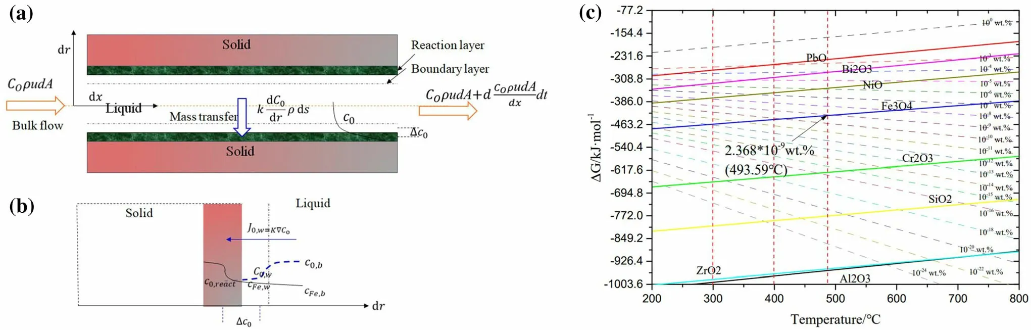
Fig. 2 (Color online) Mass transfer model: a oxygen transport in the control volume, b the oxygen transport process on the surface of the substrate, and c the Ellingham diagram

When the oxygen concentration in the loop was high or temperature was low, we could only consider the oxygen consumption from iron content and assumed that the oxygen content reacted completely. It can be considered that there was almost no free oxygen in the reaction layer and,in fact, the diffusion coefficient of oxygen in the reaction layer was very low; thus, it can be considered that CO,re-<<CO,b. The concentration of iron at the interface between the fluid and solid was much lower than that in the reaction layer (usually considered equal to the saturation concentration). Moreover, the total iron mass flux to the reaction layer became:
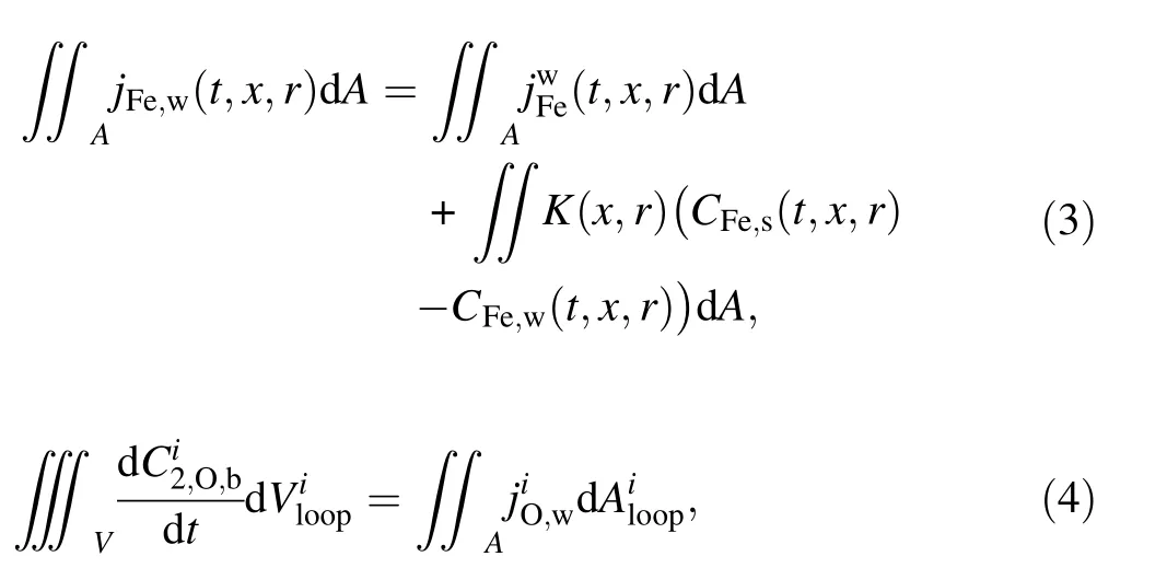
where jFe,wis the iron mass flux at the reaction surface,CFe,wis the iron concentration at the solid-liquid interface,and CFe,sis the iron concentration in the oxide layer.
Several expressions for the mass transfer coefficient in aqueous media have been developed through experimental data[21,24].Here, the Harriott and Hamilton(denoted by KHH hereafter), Berger and Hau (denoted by KBH hereafter), and Silverman models (denoted by KSi hereafter)are adopted in the following discussion.
Since the oxygen concentration on the solid side of the solid-liquid interface and the steel elements (mainly iron and the corrosion products, which were supposedly magnetite) are in a chemical equilibrium state, the following equation from Ref. [19] is given:

For the ith control volume with an oxygen source,since the volume of the oxygen source is much lower than that of the primary loop, the oxygen consumption in which the oxygen source is located can be neglected.When the valve in the oxygen control bypass is closed (corresponding to model 1),the oxygen concentration at the outlet of the first control volume can be expressed as follows:

2.3 Calculation procedure
As illustrated in Fig. 3, the calculation process of this code can be summarized in the following steps:
(1) Calculate thermohydraulic parameters at steady state.
(2) Input an initial value for oxygen and iron in bulk flow and correction factor for oxygen mass transfer coefficient, and calculate oxygen by virtue of Eqs. (7-11). Then, the iron concentration at the solid-liquid interface and in bulk flow can be calculated by virtue of Eqs. (5-6). Reset the initial value for oxygen and iron concentration in the bulk until the maximum number of iterations or relative error of the oxygen concentration obtained from two adjacent iterations is exceeded. The abovementioned process is to be repeated until values of both oxygen and iron concentrations reach a steady state.
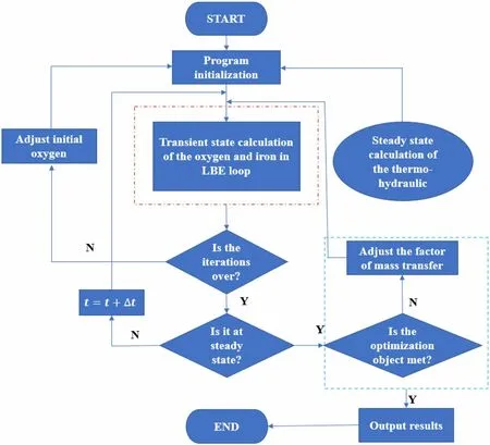
Fig. 3 Structure of the calculation code
(3) Finally, the oxygen concentration at steady state is input to the optimized calculation module. If the error between the experimental values and the simulated values exceeds the preset value, adjust the correction factor of the oxygen mass transfer coefficient. Repeat steps 2 and 3 until this requirement is met. Then, the simulation ends, and the results are the output.
In a closed loop,the periodic boundary condition for the bulk concentration of each solute is as follows:
The iteration procedure is executed until dev0 is below a predefined threshold. Here, we used the same method as the MATLIM code when calculating the iron content distribution.
3 Results and discussion
3.1 Validation of the simulation method
The applicability of the present method to other loops was validated. The correctness of the simulation method,according to the calculation process shown in Fig. 3,when it is used to simulate oxygen and iron concentration and average dissolution rate of solid PbO particles in MX as well as calculate the correction factor of the oxygen mass transfer coefficient was verified. Calculated data were compared with experimental data from CRAFT and DELTA loops [12], and following this optimized method,the revised correction mass transfer coefficient model of oxygen for pipe geometry is displayed in Table 2.
Both the calculated average oxygen concentration (the average value of the oxygen concentration at the inlet and outlet of the oxygen control system) and the dissolution rate of solid-phase PbO were compared with experimental data from the CRAFT loop [12]. As can be seen fromFig. 4, the present simulation method predicted a reliable oxygen concentration distribution and PbO dissolution rate for the CRAFT loop.

Table 2 Oxygen mass transfer coefficient K′ in (m s-1) for pipe geometry

Fig. 4 (Color online) Results of validation: comparisons of the PbO dissolution rate and average oxygen concentration in the CRAFT loop with the simulation results by the three models
3.2 Influence causes
The maximum dissolution/deposition rate, maximum corrosion depth according to 3000 h, average oxygen concentration in the equilibrium state,and time to establish the steady state of the oxygen concentration in the LBE loops are the most important parameters for discussing the performance of a solid-phase oxygen system in the LBE loop. The simulated results of the aforementioned parameters,which are based on the above-discussed three oxygen mass transfers, followed the same trend. Only the KHH mass transfer coefficient will be discussed.
3.2.1 Influence from thermal–hydraulic parameters and operating models
In the present work,the controlled variable method was used to analyze the influence of the flow rate and temperature in the main loop or in the MX for the time to establish a steady state of oxygen concentration, average oxygen concentration, maximum corrosion depth, and maximum dissolution/precipitation rate in equilibrium state. These were used to evaluate the ability to adjust the oxygen concentration in the LBE loop by the solid-phase oxygen control system and identify the operating domain in the LBE loop to meet the requirements for restriction of oxygen concentration and corrosion. The boundary conditions are displayed in Table 3, and the simulation results in Fig. 5.
As indicated in Fig. 5, the time to establish the steady state of oxygen concentration, average oxygen concentration, and maximum corrosion depth were larger under operating model 1, but the maximum dissolution/precipitation rate was lower under this model.Although under the same operating model, different influences have different effects on them.
As shown in Fig. 5a, b, the time to establish a steady state of oxygen concentration and average oxygen concentration at steady state were negatively related to flow rate in the main loop and the power of the main heater,respectively. However,as indicated in Fig. 5c,the average oxygen concentration at steady state was positively related to temperature in MX, but the time to establish a steady state has the maximum value. The following reason was accepted for this difference: this flow rate will mainly and positively affect the mass transfer coefficient of oxygen at the boundary layer [22], which means that a higher flow rate will lead to a higher consumption rate of oxygen, but the supply rate of oxygen only changes a little. Then, the time to establish a steady state and the average oxygen concentration at a steady state will decrease with the flow rate increasing,as shown in Fig. 5a.The power of the main heater in the loop will only influence the mass transfer coefficient of oxygen at the boundary layer, and the consumption rate of oxygen will increase with the increasing of the main loop’s temperature [25]. The time to establish the steady state and average oxygen concentration at the steady state in the loop will also decrease with the power of the main heater increasing, as presented in Fig. 5b. As displayed in Fig. 5c,since the oxygen concentration in the loop was mainly affected by the operating temperature in MX, the consumption rate of oxygen was the secondary cause, which was related to the oxygen concentration.Based on these influences, the oxygen concentration will increase significantly with the increasing of operating temperature in MX, especially in the high temperature region. The dissolution rate of solid PbO particles will be affected directly by the temperature and will be positively correlated with it. In addition, the consumption rate of oxygen will increase as the oxygen concentration increases(as the gradient of oxygen concentration in the boundary layer is positively related to it). Therefore, in a certain operating boundary condition, especially if the region of the operating temperature is low, the time to establish a steady state of oxygen concentration will increase with the temperature increasing at the low temperature region and then decrease with increasing temperature.
Except for the above, and as indicated in Fig. 5, the effects from flow rate and power of the main heater in the main loop and temperature in the MX on maximum corrosion depth were different.The following explanation was accepted:since the flow rate will affect both the dissolution rate of solid PbO particles and consumption rate of oxygen directly,but the main heater power only directly affects the consumption rate of oxygen, the influence on maximum corrosion depth will be slightly different. Although the gradient of oxygen concentration in the boundary layer will decrease due to oxygen concentration decreasing, the velocity will be higher and the maximum corrosion depth will increase with the flow rate increasing due to an increased mass transfer coefficient [22], as displayed in Fig. 5a. Moreover, there will be a smaller decrease with main heater power increasing when the main heater power is lower than 5 kW due to the decreased gradient of the oxygen concentration in the boundary layer and the temperature in the loop being low.However,the mass transfer coefficient of oxygen will increase with an increase in temperature[21].Then,the maximum corrosion depth willslightly increase when the main heater power is 8 kW, as indicated in Fig. 5b.

Table 3 Boundary conditions under two operating models

Fig. 5 (Color online) The distribution of time to establish steadystate oxygen concentration, average oxygen concentration in loop,and the maximum corrosion depth with different thermal-hydraulic parameters under two operating models: a influence from the flow rate in the main loop,b influence from the power of the main heater in the main loop, and c influence from the temperature in the MX.Distribution of the maximum dissolution/precipitation rate with:a main loop with flow rate,b main heater power in the main loop,and c temperature in the MX under two operating models
To illustrate the effects of the above cases, the maximum dissolution/precipitation rates under different boundary conditions are displayed in Fig. 5d-f. As illustrated in previous studies [19-22], the dissolution/precipitation rate is negatively correlated with oxygen concentration in the loop, but positively correlated with loop temperature. Therefore, based on the above analysis,it increased with the main loop flow rate and main heater power increasing (Fig. 5d, e) and decreased with MX temperature increasing (Fig. 5f).
This new understanding of the dependence of time to establish a steady-state oxygen concentration, average oxygen concentration, maximum corrosion depth, and maximum dissolution/precipitation rate on the flow rate and temperature in the loop or MX is beneficial for designing and operating non-isothermal closed LBE loops.We plan to verify the key aspects in future experiments.This dependence implies that the results obtained from one loop cannot be fully and directly applied to another loop with different operating boundary conditions.
The bulk oxygen and iron concentrations along the LBE loop,which correspond to the above operating models,are presented in Fig. 6.Notably,changing the operating model of the solid-phase oxygen control system does not cause a significant difference in the distribution of oxygen along the loop.However,a significant difference was observed in the overall oxygen and iron concentration levels in the loop due to a different supply rate of oxygen by PbO particles,and the overall oxygen in the loop was higher than that under model 2. Meanwhile, the iron concentration at the solid-liquid interface was negatively corrected with the oxygen concentration [19-21], and the iron concentration will be lower.
3.2.2 Operation domain
In the long-term operation of the LBE loop, the oxygen concentration in the loop must meet the requirements of the upper and lower limits. According to the thermodynamic criteria for oxygen control in LBE, the limit has been discussed in detail in the LBE handbook.An active oxygen control for corrosion protection by iron oxide film corresponds to the narrow area delimited by the PbO line(upper limit) and Fe3O4line (lower limit). Therefore, we decided to work with the following expression for the upper limit oxygen concentration obtained from Gromov et al. [26]:
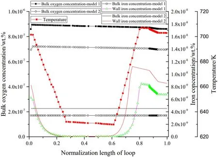
Fig. 6 (Color online) One-dimensional distribution of iron and oxygen concentrations under two different operating models
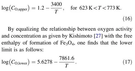
The allowable maximum oxygen concentration in the non-isothermal loop can be considered equal to the saturated oxygen concentration, which corresponds to the lowest temperature in the LBE loop, and the allowable minimum can be considered equal to the oxygen concentration used to format the protected oxide film (Fe3O4) at the highest temperature point. Following Eqs. (16 and 17),the corresponding oxygen concentration limits in our nonisothermal LBE loop when its main heater power is 0.5 and 8 kW are summarized in Table 4.The allowable operating domain of the oxygen concentration was between 2.2459 × 10⁻¹¹wt% and 6.159 × 10⁻⁵wt% (heater power 0.5 kW) and between 2.368 × 10⁻⁹wt% and 6.4832 × 10⁻⁵wt% (heater power 8 kW), respectively.
A cloud map of the average oxygen concentrations with the main loop flow rate and temperature in MX under main heater powers of 0.5 and 8 kW are displayed in Fig. 7a, b.Based on the analysis of Fig. 5b, it can be concluded that the operating boundary of this loop, as shown in Table 4,meets the loop’s requirements for oxygen concentration limits.
Meanwhile,the loop also needs to meet the requirement for allowable maximum corrosion depth. Based on the above-calculated results for maximum corrosion depth and dissolution/precipitation under two operating models and boundary conditions as summarized in Table 4, both the maximum corrosion depth and dissolution/precipitation under model 1 will be higher than those under model 2.Therefore, in the present work, the allowable maximum corrosion depth in the loop was taken as one of the criteria,and only operating model 1 was considered.Assuming that the allowable maximum corrosion depth in the loop was 6 μm (3000 h)-1, the cloud diagrams of allowable corrosion depth with main loop flow rate and operating temperature in MX when the main heater power was 0.5 and 8 kW are displayed in Fig. 7c, d, respectively. Based on the analysis of Fig. 5b, when the main heater power was between 0.5 and 8 kW, the safety operating domain in our non-isothermal LBE loop can take the common domain,as displayed in Fig. 7e. When the main heater power is between 0.5 and 8 kW,the allowable temperature in MX is 640 K, and if it is higher than 573.15 K, the allowable maximum flow rate in the main loop is 2.8125 kg s-1.

Table 4 Oxygen concentration limits based on Eqs.(16 and 17)

Fig.7 (Color online)Cloud map of the average oxygen concentration or allowable operating domain in the loop under main heater powers of 0.5 or 8 kW and the safety operating domain
4 Conclusion
In summary, a specific simulation method for corrosion was proposed for non-thermal LBE loops equipped with solid-phase oxygen control systems. Combining with the dissolution model of PbO, the above method was intended to optimize the prediction of the one-dimensional distribution of oxygen and iron concentrations and predict the maximum dissolution/precipitation rates of corrosion products as well as the maximum corrosion depth in the entire LBE loop. This method was also applied to CRAFT and DELTA loops. Comparisons between the calculated results and experimental data indicated that the present method exhibited satisfying applicability to other LBE loops and can produce a reliable simulation result. Most importantly, the effect of the operating model of the oxygen control system and thermohydraulic parameters in the loop on the above parameters is discussed based on the present optimized method. Primary findings can be concluded as follows:
(1) A safety operating domain of our LBE loop was found (Fig. 6e) when the main heater power was between 0.5 and 8 kW.
(2) The average oxygen concentration at steady state under operating model 1 was higher and the time to establish steady state was relatively longer. As indicated in Fig. 5c, increasing the temperature in MX is the most efficient and optimal step to regulate the oxygen concentration in the loop,and a heater or cooler in the oxygen control system is needed.
Author contributionsAll authors contributed to the study conception and design. Material preparation, data collection, and analysis were performed by Xiao-Bo Li, Rui-Xian Liang, Yi-Feng Wang,Hui-Ping Zhu, Fang Liu, Yang Liu, Cong Li, Hao Wu, and Feng-Lei Niu.The first draft of the manuscript was written by Xiao-Bo Li,and all authors commented on previous versions of the manuscript.All authors read and approved the final manuscript.
杂志排行

Nuclear Science and Techniques的其它文章
- Design and tests of the prototype a beam monitor of the CSR external target experiment
- Development of a wide-range and fast-response digitizing pulse signal acquisition and processing system for neutron flux monitoring on EAST
- On the viability of wearing evaluation by Thin Layer Activation in the presence of non-occupationally exposed individuals
- Enhancement in optical absorption of CsI(Na)
- Research on tune feedback of the Hefei Light Source II based on machine learning
- Development of a subchannel code for blockage accidents of LMFRs based on the 3D fuel rod model