Iterative Identification of Robot Dynamic Parameters Based on Logistic Function

，*，，，，，

1. College of Mechanical & Electrical Engineering，Nanjing University of Aeronautics and Astronautics， Nanjing 210016， P. R. China；

2. Key Laboratory of Digital Manufacturing Aviation Technology， AVIC Aeronautical Technology Institute，Beijing 100024， P. R. China

Abstract: The dynamic parameter identification of the robot is the basis for the design of the controller based on the dynamic model. Currently， the primary method for solving angular velocity and angular acceleration is to filter and smooth the position sequence and then form a differential signal. However， if the noise and the original signal overlap in the frequency domain， filtering the noise will also filter out the valuable information in the frequency band. This paper proposes an excitation trajectory based on Logistic function， which fully uses the information in the original signal and can accurately solve the angular velocity and angular acceleration without filtering and smoothing the position sequence. The joint angle of the excitation trajectory is mapped to the joint angular velocity and angular acceleration one by one so that the joint angular velocity and joint angular acceleration can be obtained directly according to the position. The genetic algorithm is used to optimize the excitation trajectory parameters to minimize the observation matrix’s condition number and further improve the identification accuracy. By using the strategy of iterative identification， the dynamic parameters identified in each iteration are substituted into the robot controller according to the previous position sequence until the tracking trajectory approaches the desired trajectory， and the actual joint angular velocity and angular acceleration converge to the expected value. The simulation results show that using the step-by-step strategy， the joint angular velocity and joint angular acceleration of the tracking trajectory quickly converge to the expected value， and the identification error of inertia parameters is less than 0.01 in three iterations. With the increase of the number of iterations， the identification error of inertial parameters can be further reduced.

Key words：robot； dynamic parameter identification； Logistic function； iterative identification； excitation trajectory

0 Introduction

The development and production of the new generation of aerospace products put forward higher new requirements for manufacturing accuracy and processing quality. Intelligent manufacturing technology and equipment with the robot as the core is an effective way to solve this problem［1-4］. Currently， most robots use proportional integral differential control （PID）， which leads to low trajectory tracking accuracy in the case of high speed and heavy load， so it could not be well applied in the aerospace field. The design of the motion controller based on the robot dynamics model is an effective way to realize high-speed and high-precision motion control.

The robot is a nonlinear system with strong coupling and multivariable， and the dynamic parameters are difficult to be measured accurately. In order to establish an accurate dynamic model of the robot， it is necessary to identify its parameters［5-6］.

Robot dynamic parameter identification generally includes the following steps： dynamic modeling， excitation trajectory design， data sampling and processing， solution of angular velocity and angular acceleration， parameter identification， and model verification. The accuracy of angular velocity and angular acceleration determines the accuracy of parameter identification. If the method of numerical differentiation of the joint angle is adopted， high-frequency noise will be introduced， and the angular velocity and angular acceleration signals cannot be used for parameter estimation. Atkeson et al.［7］used finite polynomial series as the excitation trajectory and proposed to estimate the joint angular velocity and angular acceleration by filtering the position signal. However， there is a certain phase delay in the filtered joint angular velocity and joint angular acceleration signal. Kinsheel et al.［8］made a high-precision central finite difference for the position sequence to obtain a more accurate joint angular velocity. However， the estimation of the joint angular acceleration is still affected by noise. On the other hand， Swevers et al.［9］used the finite term Fourier series as the excitation trajectory and proposed two methods to obtain the joint angular velocity and joint angular acceleration： （1） The measured position could be approximated by a finite Fourier series containing the same limited set of frequencies as the desired position. （2） Due to the periodicity of the measurements， the velocity and acceleration could be calculated in the frequency domain after Fourier transform. There is a certain leakage error in these two methods because the finite Fourier series is used to fit the actual trajectory. Xu et al.［10］smoothed the joint acceleration and torque after calculating the joint velocity and acceleration through the central difference algorithm in the experiment. Zhang et al.［11］modeled the robot with harmonic reducers and identified the parameters of the model， five spot triple smoothing method was applied to the torque signal， and low-pass filtering was applied to solve the angular velocity and angular acceleration obtained from the difference. Feng et al.［12］proposed an identification method based on the iterative reweighted least square algorithm. The weight coefficient matrix is formed by adding measurement torque noise， and the reciprocal of torque noise is used as the weight coefficient to improve the identification accuracy. In terms of the solution of angular velocity and angular acceleration， the angular velocity is obtained by filtering， and the angular velocity is fitted into Fourier series form. The joint angular acceleration is obtained by differentiating the Fourier series of the joint angular velocity.

From the above research， it can be concluded that the current mainstream methods for solving angular velocity and angular acceleration are still filtering， smoothing， fitting， central difference， or a combination of these methods. These methods will filter out the original signal in the same frequency band as the noise while eliminating the noise and may also cause the phase delay and waveform distortion of the original signal. This paper proposes an excitation trajectory based on Logistic function， which fully uses of the information in the original signal and can accurately calculate the joint velocity and acceleration without denoising. The trajectory maps the joint angle of the excitation trajectory to the joint angular velocity and joint angular acceleration one by one， so that the robot excitation trajectory satisfies the flexible start and stop conditions， at the same time， the joint angular velocity and angular acceleration can be directly obtained by the expression with joint angle variables. On the other hand， in the existing identification methods， the robot only runs the excitation trajectory once. The dynamic model of the robot is unknown before the running trajectory， so the tracking error of the excitation trajectory is significant， and there will be a large rounding error when fitting the actual trajectory with the analytical formula of the expected excitation trajectory. The iterative identification method is adopted in this paper. After identifying a group of parameters， the identified parameters are substituted into the controller to make the robot joint track the trajectory more accurately， and the more accurate tracking trajectory can identify more accurate parameters. The parameters continue to be substituted into the controller to perform the above steps iteratively. Finally， the angular velocity and angular acceleration of the actual tracking trajectory converge to the expected value， and the parameter identification accuracy is further improved.

1 Dynamic Modeling of Robot

For the robot withndegrees of freedom， the dynamic equation is obtained by the Newton Euler method or Lagrange method

whereq∈Rn，˙∈Rn，¨∈Rnare the robot joint position vector， the joint velocity vector， and the joint acceleration vector， respectively.M(q)∈Rn×nis then×nmass matrix，C(q，˙)∈Rnthe centrifugal force and gothic force vector，G(q)∈Rna gravity term，τr∈Rnthe input moment vector for the joint， andτf∈Rnthe joint friction torque vector. The inertia parameter vector of connecting rodican be expressed aspi=[mi，mirxi，miryi，mirzi，Ixxi，Ixyi，Ixzi，Iyyi，Iyzi，Izzi]T，heremiis the mass of the rodiandrci=[rix，riy，riz] the expression of the center of mass of the rodiin the coordinate system｛i｝；Ixxi、Ixyi、Ixzi、Iyyi、Iyzi、Izziare the items in the inertia tensor. Eq.（1） can be converted into the linear form of inertial parameters［13］.

whereP=[pT1，pT2，pT3，…，pTn]T∈R10n×1is the inertia parameter ofnjoints of the robot.κ(q，˙，¨)∈Rn×10nis the corresponding regression matrix， and each item in the matrix is a function of joint angle， angular velocity， and angular acceleration. Some elements in vectorPare redundant to the dynamic model （the corresponding coefficient is zero）， and these elements cannot be identified. Some elements need to be identified by linear combination as a whole. By eliminating or reorganizing these elements， the minimum set of identifiable parameters can be obtained， which is usually called the minimum inertia parameter. Kawasaki et al.［14］gave a recursive formula for completely determining a set of inertia parameters of the robot by using the modified DH parameters. On this basis， Huo et al.［15］gave a set of simpler recursive formulas， so the dynamic model of the robot can be expressed as a linear form of the minimum inertia parameter set. The joint friction torque vectorτfcan be described by the C-V model［16］or stribeck model［17-18］， the parameters in the model can be identified in advance. In this paper， it is assumed that the joint friction model is known and the joint friction torque vectorτfcan be obtained. Letτ=τr-τf，τcan be given by

whereΦ(q，˙，¨)∈Rn×mis an observation matrix andθ∈Rm×1(m＜10n) the minimum inertia parameter vector.

In this paper， the two-degree-of-freedom（2-DOF） robot in the vertical plane is taken as the object to study the iterative identification of the dynamic parameters， and this kind of robot can be used for handling and assembling. In addition， the research on the 2-DOF robot will pave the way for the research on robots with more degrees of freedom. The D-H model of the robot is shown in Fig.1， and the modified D-H parameters of the robot are shown in Table 1.

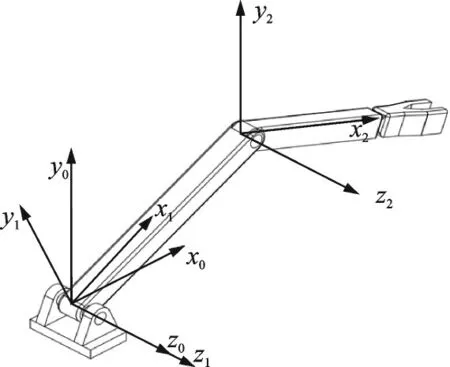
Fig.1 Modified D-H model of the robot

Table 1 Modified D-H parameters of the robot

In Table 1，αi-1is the （i-1）th rod torsion angle，ai-1the length of rodi-1，dithe offset of rodi， andqitheith joint angle. According to the recursive formula in Ref.［15］， the minimum inertia parameters are shown in Table 2.

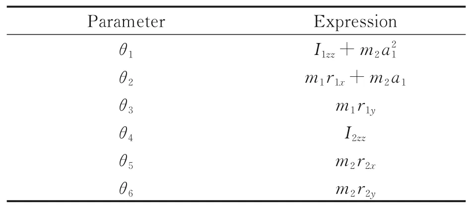
Table 2 Minimum inertia parameter set of 2-DOF robot kg·m2

For the 2-DOF robot， the Lagrangian dynamic equation is listed as follows

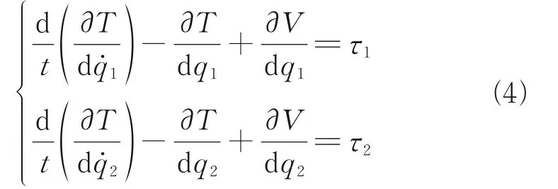
whereTis the sum of the kinetic energy of each rod andVthe sum of the gravitational potential energy of two rods. The expressions ofTandVare listed as follows

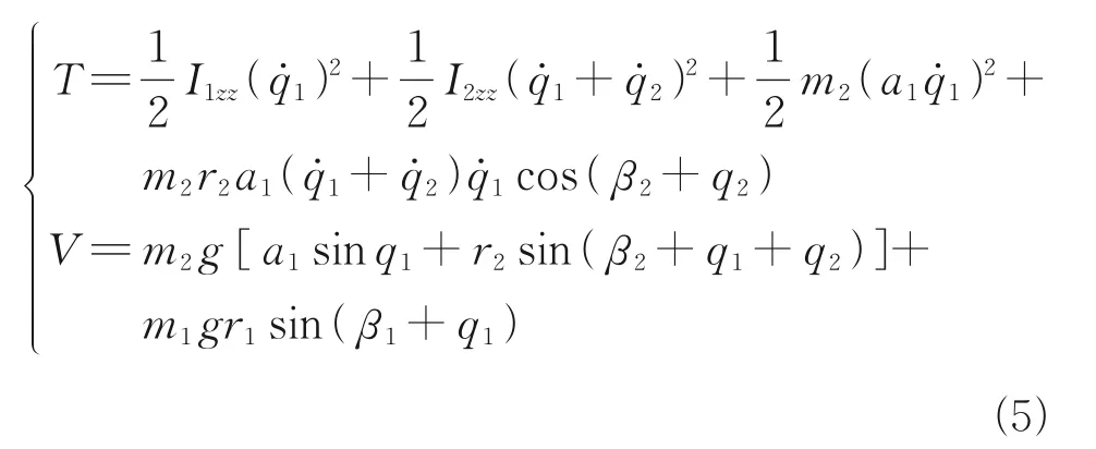
whereβi=arctan(rix/riy)，[rix，riy，riz] is the coordinate of the centroid of the rodiin theith joint coordinate system. Substituting Eq.（5） into Eq.（4） yields

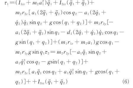
The observation matrix can be obtained by extracting the minimum inertia parameter set in Table 2 from Eq.（6） in the form of Eq.（3） and the expression of the observation matrix is as follows

whereφ11=，φ12=gc1，φ13=-gs1，φ14=¨+¨，φ15=a1(¨+)c2-a1(+˙)˙s2+gc12，φ16=-a1(¨+)s2-a1(˙+)˙c2-gs12，φ21=0，φ22=0，φ23=0，φ24=+¨，φ25=gs12. Among them，s1=sinq1，c1=cosq1，s2=sinq2，c2=cosq2，s12=sin(q1+q2)，c12=cos(q1+q2)，gis the acceleration constant of gravity.

LetM=[φ11φ12φ13]，N=[φ14φ15φ16]，Q=[φ24φ25φ26]， the observation matrixΦcan be expressed as

Eq.（3） can be written as

The identification process can be divided into the following two steps：

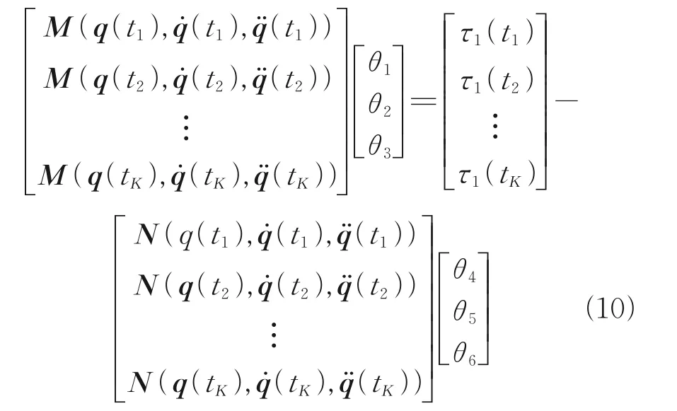
Step 1By making joint 1 rest and joint 2 move， and takingKsamples of joint angle and torque at timet1，t2，…，tK， the following equation can be obtained

whereQ(q(tK)，˙(tK)，¨(tK)) is the observed value of matrixQat timetKandτ2(tK) the driving moment value of joint 2（excluding friction torque） at timetK.θ4，θ5，andθ6can be obtained by the least square method.

Step 2Afterθ4，θ5，θ6have been identified， by making joint 2 rest and joint 1 move， and takingKsamples of joint angle and torque at timet1，t2，…，tK， the following equations can be obtained

2 Design of Excitation Trajectory

2.1 Excitation trajectory based on Logistic function

In order to calculate the observation matrix， the angular velocity and angular acceleration information need to be estimated by the joint angle sequence. if the method of numerical differentiation of joint angle is used， high-frequency noise will be introduced. The angular velocity and angular acceleration signals cannot be used for parameter identification. Therefore， a kind of trajectory can be used， in which the joint angle is mapped to the joint angular velocity and joint angular acceleration one by one. Under the condition of accurate trajectory tracking， the angular velocity and angular acceleration can be obtained by bringing the angle directly into the analytical formula. As a result， the interference of the high-frequency noise is avoided and the identification accuracy is improved.

On the other hand， the excitation trajectory needs to meet flexible start-stop conditions. At the beginning and end of the test， sudden changes in velocity and acceleration may lead to robot flutter， which makes it difficult to track the trajectory accurately and reduce the accuracy of parameter identification. The flexible start-stop condition of the excitation trajectory can be expressed as follows

whereqinitis the initial joint angle vector of the robot andtfa cycle of movement. At the end of one motion cycle， the robot returns to its initial position and continues the next cycle of movement. In order to meet the above conditions， the Logistic function is used here， and its expression is as follows

For the Logistic function， the following two equations hold：f′(t)=f(t)[1-f(t)]，f′(t)=f(t)[1-f(t)][1-2f(t)]. The function image with domain （-10，10） is shown in Fig.2.

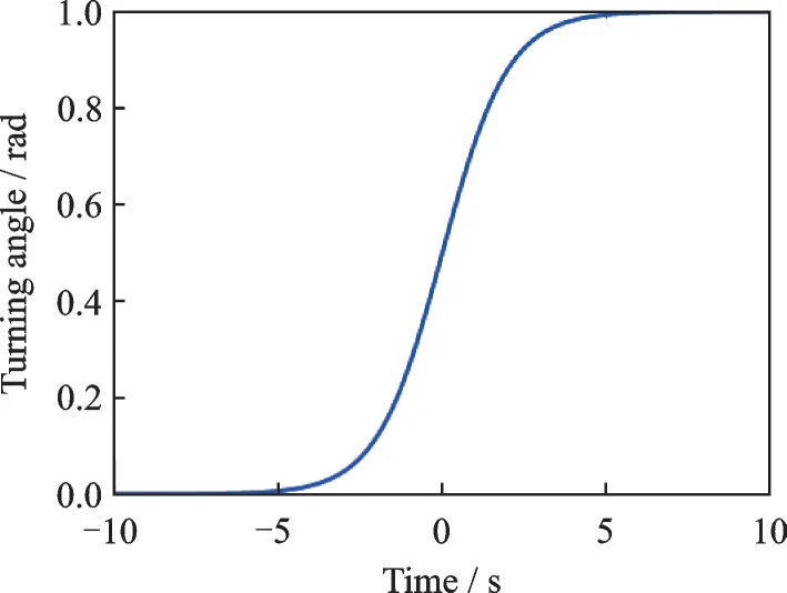
Fig.2 Logistic function

When the function is spliced into the trajectory of the robot joint shown in Fig.3， at the beginning： |˙(0)|=|f′(-10)|＜10-4，||¨(0)=|f′(-10)|＜10-4， at the end of the period：||˙(tf)=|-f′(10)|＜10-4， |¨(tf)|=|-f′(10)|＜10-4，and at the splicing of the trajectory： ||(20)， |(20)|，|(20)|，|(20)|＜10-4， which means the angular velocity and angular acceleration of the trajectory at the beginning， end， and splicing are almost zero， so it can be considered that the flexible start-stop condition is satisfied.

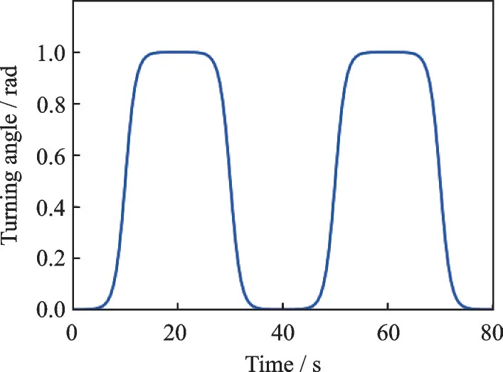
Fig.3 Spliced Logistic function

Add the adjustable parametersA，w，φ，hto the Logistic function to change it to the formf*(t)=Af(wt+φ)+h，f*(t) can be expressed as

The functionf*(t) is spliced into the excitation trajectory withTas the period， and the expression of the excitation trajectory after splicing is as follows

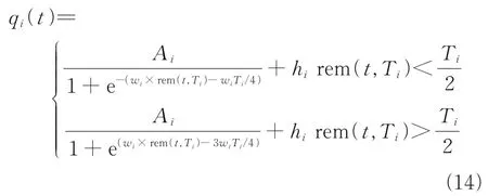
whereqi(t) is the excitation trajectory of the jointiof the robot and rem the function operation；Ai，wi，hi，Tiare the motion amplitude， the motion frequency in the period， the motion offset， and the whole motion period of jointi， respectively. The corresponding images of differentware shown in Fig.4， and the corresponding images of differentTare shown in Fig.5.

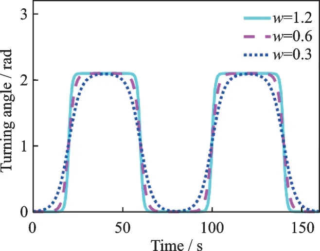
Fig.4 Function image corresponding to different w at T=80

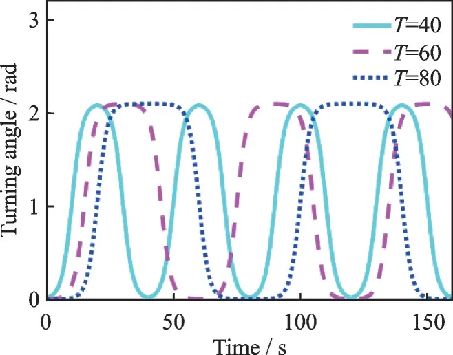
Fig.5 Function image corresponding to different T at w=0.6

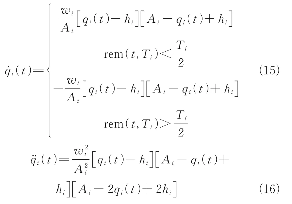
The angular velocity˙(t) and angular acceleration¨(t) of robot joints can be expressed by joint angleqi(t)

2.2 Optimization of excitation trajectory

In order to improve the identification accuracy， it is necessary to select the appropriate index function to optimize the excitation trajectory. The condition number of the observation matrix reflects the convergence rate of the parameter estimation of the anti-noise ability of the identification method［7］. Not all sampling points participate in the identification. The selected sampling points should minimize the number of conditions. First， find the midpoints of the start and end positions of the excitation trajectory， and mark the coordinates of these points as

wheretmkis the Abscissa of thekth midpoint andnthe total number of midpoints. The part involved in the identification is the neighborhood of these points， that is， the solid part in Fig.6. The range of the Abscissa of this part ist∈(tmk-δ，tmk+δ)，k=1，2，…，n， whereδis the radius of the neighborhood centered ontmkand needs to be further optimized.

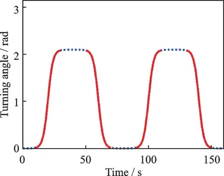
Fig.6 Areas involved in the identification

The optimization problem of excitation trajectory based on the condition number criterion can be described as

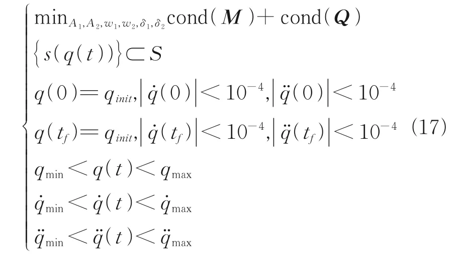
where cond(M)，cond(Q) are the condition numbers of matrixMandQ，respectively， and {s(q(t))} is the set of terminal positions when the robot tracks the excitation trajectory， which can be calculated by forward kinematics.sis the workspace of the robot， andare the constraint value of the joint angle， angular velocity， and angular acceleration. Eq.（17） is a nonlinear constraint problem， which can be optimized by genetic algorithm. Taking the 2-DOF series robot as an example， assuming that the set of the terminal position of the end of the robot is above the ground， the angular velocity of each joint does not exceed π/6(rad/s)， the angular acceleration of each joint does not exceed π/15(rad/s2)， and the starting position of each joint is 0， then there are the following constraints

Genetic algorithm is used to solve the above optimization problems， and the fitness function is taken as follows

whereεis the value of reward and punishment， and if the constraint condition is satisfied，ε=0； if the constraint condition is not met，ε=1 000.The objective of optimization is to minimizeH， so the probability of each gene being selected is 1/H. The individuals in the genetic algorithm are encoded in binary， the binary digits are 20， and the variable dimension is 6. Since the dimension of the variable to be solved is not high and it is not easy to fall into the local optimal solution， the initial population number can be set to 40. In genetic algorithm， the range of crossover probability is usually 0.1─0.5， and the range of mutation probability is 0.001─0.05. It is found that when the crossover probability is 0.5 and the mutation probability is 0.01， the convergence speed of genetic algorithm is faster and the solution result is better. After 500 generations， the optimal solution is no longer updated and the model converges， so the optimization algebra is taken as 500. The detailed steps of genetic algorithm can be found in Ref.［19］， the fitness function curve of the optimization process is shown in Fig.7， and the optimized trajectory parameters are shown in Table 3.

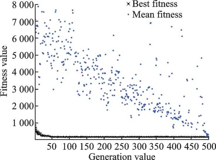
Fig.7 Optimization process

Table 3 Optimized trajectory parameters

3 Iterative Identification and Simulation

In the case of accurate trajectory tracking， because the joint angular velocity and angular acceleration are obtained by the angle sequence directly into the analytical formula， the interference of high-frequency noise is avoided and the identification accuracy is improved. If the trajectory tracking is not accurate， a group of parameters can be identified first. The identified parameters are substituted into the controller to enable the robot joint to track the trajectory more accurately， and the more accurate tracking trajectory can identify more accurate parameters. The parameters continue to be iterated into the controller to carry out the above steps， so that each tracking trajectory is closer to the desired trajectory， and the actual joint angular velocity and joint angular acceleration converge to the expected value. In this paper， the iterative identification simulation of a 2-DOF robot is carried out， assuming that the rod length isa1=1， and the inertia parameter isθ=[ 2，2，0，1，1，0]T. The process is shown in Fig.8.

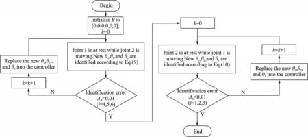
Fig.8 Parameter identification process

The identification error in Fig.8 is the absolute value of the difference between the identified value of the inertia parameter and the given value of the inertia parameter in the simulation，namely

whereΔikis thekth identification error of theith inertial parameter，θikthekth identification value of theith inertial parameter， andθidthe given value of theith inertial parameter in the simulation.

The controller needs to use the control algorithm based on robot dynamics， and the robustH∞finite time algorithm［20］is adopted here. RobustH∞control is a kind of controller with fixed structure and parameters， which has the ability to deal with disturbances， fast-changing parameters and final modeling dynamics. It can make the designed controller meet the design requirements even when the uncertainty is the most serious damage to the quality of the system. Define Sig(·)α∈Rn，shown as

whereξ=[ξ1，ξ2，…，ξn]T∈Rn，0＜α＜1，sgn(·) is a symbolic function， defined as follows

RobustH∞finite time control （RHFTC） can be described as

whereqdis the second-order derivable desired trajectory， andandare its first derivative and second derivative， respectively.qis the actual trajectory，eis the trajectory tracking error，e=qd-q˙=-˙，andα2=2α1/α1+1. The parameters of joint 1 are set toKp1=2，Kd1=20， and the parameters of joint 2 are set toKp2=4，Kd2=4.α1=0.7，α2=0.82.

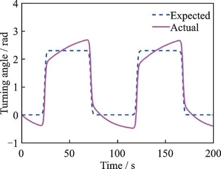
Fig.9 The first tracking trajectory of joint 2

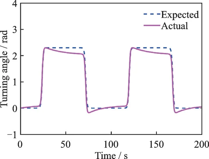
Fig.10 The second tracking trajectory of joint 2

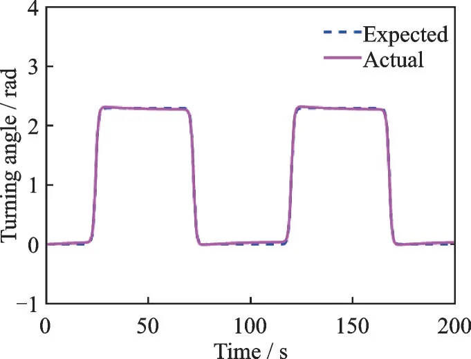
Fig.11 The third tracking trajectory of joint 2

Using the step-by-step identification strategy， first let joint 1 rest and joint 2 moves， and the actual trajectory of joint 2 in the first three times is shown in Figs.9─11. At the beginning， the actual trajectory fluctuates up and down near the desired trajectory， and the fluctuation range is large. After one iteration， the actual trajectory still fluctuates up and down near the expected trajectory， and the fluctuation amplitude is significantly reduced compared with the first iteration. After another iteration， the actual trajectory almost coincides with the expected trajectory. The tracking erroreof joint 2 in the first three times is shown in Fig.12.The maximum tracking error of the first iteration can reach 0.6 rad. After one iteration， the maximum tracking error is 0.15 rad， which is only 25% of the first iteration. After another iteration， the tracking error converges to 0. The inertia parameter identification values of joint 2 in the first three times are shown in Table 4. It can be seen that the identification error of the inertia parameterθ4is the largest. At the beginning， the identification error can be as large as 0.7. After three iterations， the maximum identification error is reduced to 0.007， which is a relatively small value.

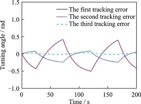
Fig.12 Tracking error of the first three times of joint 2

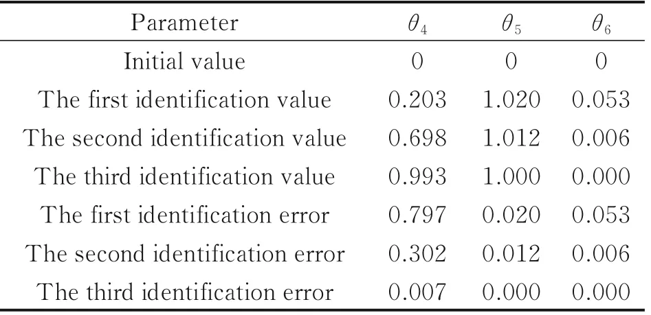
Table 4 Inertial parameter identification values of the first three times of joint 2

Afterθ4，θ5，andθ6have been identified， make joint 2 rest and joint 1 move， and the first three tracking trajectories of joint 1 are shown in Fig.13. The first three tracking errors of joint 1 are shown in Fig.14. Similiar to joint 2， after the third iteration， the error converges to 0. The first three inertial parameter identification values of joint 1 are shown in Table 5. After three iterations， the identification error of the inertia parameterθ1is the largest， and the maximum identification error is only 0.009， which is also a relatively small value.

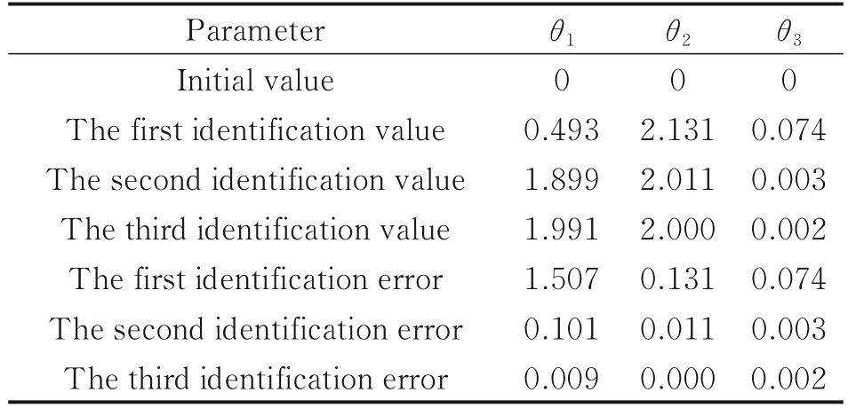
Table 5 Inertial parameter identification values of the first three times of joint 1

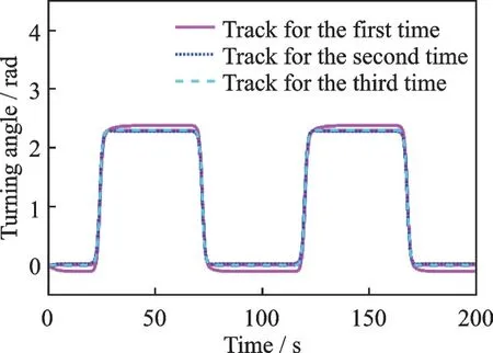
Fig.13 Track of joint 1 for the first three times

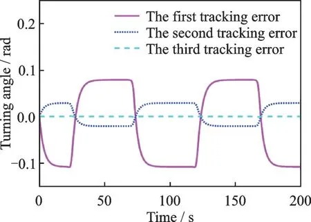
Fig.14 Tracking error of joint 1 for the first three times

The simulation results show that for the 2-DOF series robot， the step-by-step iterative identification strategy has good convergence for both the first joint and the second joint， and the identification errors of all inertia parameters are less than 0.01 after three iterations. If the number of iterations is increased， the progress of identification can be further improved. The algorithm is easy to implement and has high identification accuracy.

In order to further analyze the accuracy of Logistic iterative identification algorithm， in this paper， the dynamic parameters identified by finite Fourier series trajectory and Logistic function trajectory are substituted into the dynamic model respectively. The moment of each joint in the motion process is predicted through the position sequence and compared with the actual driving moment of the robot. The modern parameter identification generally adopts the finite Fourier series， as shown in

whereqi，0is the initial position offset of the joint；wfthe fundamental frequency of Fourier series；Hthe highest order of Fourier series； andkthe order of Fourier series.ai，k，bi，kare the coefficients of Fourier series of theith joint. The specific steps for the design and optimization of Fourier series trajectories can be found in Ref.［9］. The optimized Fourier series trajectories are shown in Fig.15， and the identified parameters are shown in Table 6.

Table 6 Inertia parameters identified by Fourier series

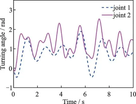
Fig.15 Optimized Fourier series trajectories

In order to test the generalization ability of the model substituted with the identification parameters， the original identification trajectory cannot be used as the verification trajectory， so this paper selects another different trajectory as the verification trajectory.

whereqi(t) is the excitation trajectory of jointiof the robot. The position sequence and driving torque of the robot can be sampled in the simulation process. The corresponding predicted torque can be obtained by substituting the position sequence of the verification track and the identified parameters into the dynamic model （Eq.（3））. The predicted torque and driving torque of joint 1 are shown in Fig.16， and the predicted torque and driving torque of joint 2 are shown in Fig.17.

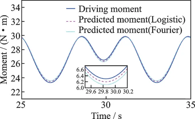
Fig.16 Predicted and driving torques of joint 1

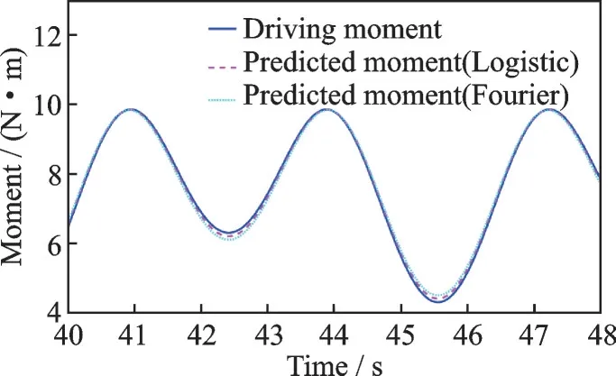
Fig.17 Predicted and driving torques of joint 2

It can be seen that the deviation between the predicted torque and the actual torque of the robot joint calculated by the two identification algorithms is relatively small， which shows the effectiveness of these two identification algorithms. In addition， it can be seen that the overall torque deviation of the identification method based on the Logistic function proposed in this paper is smaller， especially when the direction is changed， the torque deviation is significantly smaller than that of the identification method based on the Fourier series， and the overall torque curve is closer to the actual torque， that is， it has a more accurate effect on the dynamics prediction of the robot.

4 Conclusions

（1） The one-to-one mapping between the joint angle of the excitation trajectory and the joint angular velocity and joint angular acceleration is the prerequisite for iterative identification. The excitation trajectory based on Logistic function is proposed， which satisfies the flexible start and stop condition while mapping joint angle to joint angular velocity and joint angular acceleration.

（2） The condition number reflects the sensitivity of the matrix calculation to the error. The genetic algorithm is used to optimize the parameters of the excitation trajectory to minimize the condition number of the observation matrix， so as to further improve the identification accuracy.

（3） An iterative identification strategy is proposed， in which the joint angular velocity and joint angular acceleration are calculated according to the mapping relationship in each iteration， and the identified dynamic parameters are substituted into the robot controller so that the next tracking trajectory is closer to the desired trajectory. The simulation results show that using the step-by-step strategy， the joint angular velocity and joint angular acceleration of the tracking trajectory quickly converge to the expected value， and the identification error of inertia parameters is less than 0.01 in three iterations. With the increase of the number of iterations， the identification error of inertial parameters can be further reduced.