Study on Ice Load Inversion Based on LSTM Networks
2021-12-31-,-,-,
-,-,-,
(1.China Ship Scientific Research Center,Wuxi 214082,China;2.College of System Engineering,National University of Defense Technology,Changsha 410000,China;3.Bureau Hyperborea,Saint Petersburg 190000,Russia)
Abstract: Precise measurement of ice loads in actual navigation has not been worked out well for a long time. To solve the problem better, a new method of ice load inversion based on data is proposed in the paper. The training data to establish the inversion model are generated by finite element calculation. The process of training data generation is described explicitly. The structures of LSTM networks are optimized by the refined grey wolf optimizer algorithm. A valid ice load inversion model based on LSTM networks is trained successfully. The general conclusions and results are illustrated by the concrete calculation samples.
Key words:ice load;inversion problem;deep learning;LSTM networks;grey wolf optimizer algorithm
0 Introduction
Precise determination of loads[1-2]is always a hot issue in the field of structure. For objectives with relative movements, setting mechanical sensors in the contact point is the most effective measure. However, the contact points are not determined easily in the process of ship ice interaction[3],owing to the randomness and uncertainty of ice loads. We can only use the response of the given structure points to distinguish the load,such as stress,strain,displacement and so on.
The traditional measures of inversion has been applied in engineering widely,such as time-domain method and frequency-domain method. Liu[4]has inverted the ice load with the regularization method,obtaining the analytical formula in simplified structure model.
This paper presents a new method of ice load inversion based on data, which contains two parts,direct problem and inverse problem.The direct problem needs to predict the ice loads,and to calculate the dynamical response of ship structure in time domain. The predicting values of ice loads are determined by the given natural environmental information. The direct problem generates a mass of original data by inputting different environmental information. The inverse problem uses the above original data to train an LSTM network to fulfil a nonlinear mapping from the dynamic response of ship structure to the average ice loads in time domain.The work trains a successful LSTM network that gains a good result in test data eventually.
1 Direct problem
The direct problem is the foundation of the inverse problem. The direct problem needs to predict the ice loads,and to calculate the dynamical response of ship structure in time domain.The direct problem generates a mass of original data by inputting different environmental information.Only when the original data are credible, could the inverse problem establish a valid nonlinear mapping from the dynamic response of ship structure to the average ice loads in time domain.So as a result of shortage of experimental data or actual measurements, the validity of the direct problem exerts a significant influence on the accuracy of inversion model.
1.1 Natural environment of designed ships
When an ice-ship is in its preliminary design stages, the designer must confirm ice condition of a given sea area. The ice condition is the most important natural environment information in the process of predicting ice loads. Only after the above data have been mastered, could the designed ice load be calculated with combination of Ice Class and ship’s principle dimensions.
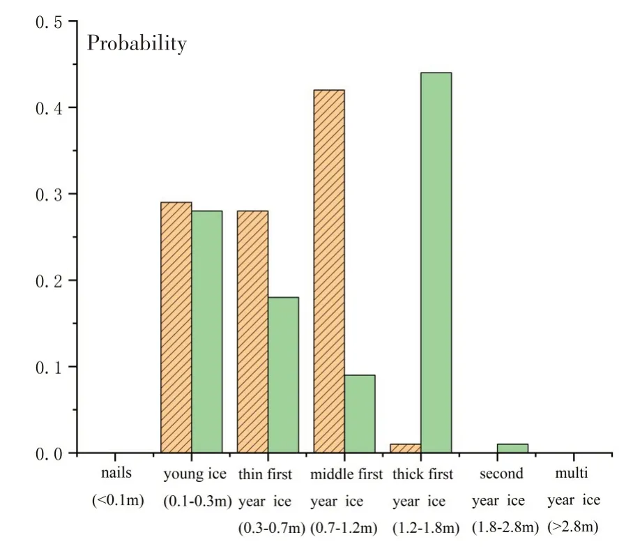
Figs.1-2 give the examples of partial distributions bar charts for ice cover thickness and for snow cover thickness plotted for February.The two ship navigation routes are Kloguev Island-Kara Gate Strait-Dickson Island (dashed lines) and Decision Island-Vilkitsky Strait-Khatanga River Mouth(solid lines)[5].

Fig.1 Partial distributions bar chart for ice cover thickness in February

Fig.2 Partial distributions bar chart for snow cover thickness in February
A dangerous scenario of a low probability will be selected as the designed scenario in the given navigation routes.Thus,an ice cover of 2 m thick and a snow cover of 0.5 m high are assumed in the paper as the typical dangerous scenario to determine the designed load.
1.2 Determination of designed ice load
The values of designed ice load recommended by ship rules and regulations were used widely during the traditional step of determining ice loads. However, the above calculating values of ice loads were usually too high in comparison with the actual situation. Hence, we use the inner ice load procedure Snow-Ice King(SIK) researched and developed by CSSRC to supply a more precise scope of ice load.
The fundamental form of principles of SIK is the dynamical energy conservation of rigid body motion,supposing that only small deformations occur in contact areas during collision.SIK uses analytical methods that combine external mechanics with ice-force function,and attains the real-time features of ice load during the collision eventually[6-7].
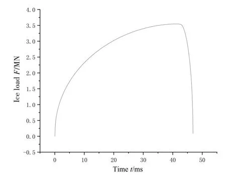
With the calculating parameters shown in Tab.1,the outcomes calculated by SIK were plotted in Fig.3 and Fig.4.The results illuminate the real-time variation of ice load in a typical calculating scenario,whose summit value is approximately about 4 MN.

Tab.1 Calculating parameters

Fig.3 Ice load in time-domain

Fig.4 Relative speed in time-domain
Fig.3 also illuminates the square wave features of ice force as one kind of impact load.To gain the dynamical response of structures in different ice conditions, it is inevitable to use the ice load curve in time domain. So in the next step, we will put different ice conditions into the SIK procedure based on the ice probability distribution.
1.3 Calculation of the dynamical responses of structures
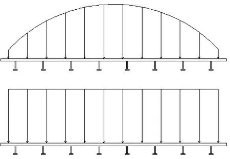
When a ship interacts with an ice flow, the crushing ice will melt and be extruded forming the inner thin layer[8], as shown in Fig.5. The existence of an inner thin layer has been testified widely in accordance with the outcomes of experiments and actual measurements. Because there exist the viscosity and plasticity among the contact area in the flowing inner thin layer,the distribution of ice load will be altered to a rather smooth parabola during the solid body penetration into the ice, as shown in Fig.6.
The mechanism of ship-ice collision load is explained by applying basic theory of the inner thin layer. The influence of nonlinear term was taken into account, and the explicit expression formula containing relative velocity was derived,as the following Eq.(1).The formula was embedded in SIK as an essential portion of ice load inversion work simultaneously.

Fig.5 Illustration of inner thin layer

Fig.6 Distribution of ice load in space

whereυis the coefficient of viscosity,ρis density,ζ˙is the relative velocity,bis the breadth of contact area,his the thickness of inner thin layer,andxis the coordinate of collision point.
This sort of ice loads’distribution will be applied in the contact areas to calculate the structural strength in the next step.
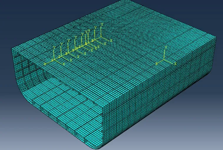
The given ship is an ice navigation vessel with the authentication of PC5.The principal dimensions of the vessel are given in Tab.1. The simplified finite element model of the ship part-cabin is established in software ABAQUS, as shown in Fig.7. The element size is generally 300 mm. The model contains 145 309 nodes and 81 633 elements,with 28 231 elements of the linear wedge type and 53 402 elements of the linear hexahedral type. The elements of the hexahedral type are more stable and nearly free of severe distortion,so this kind of elements were used as many as possible at the time of meshing models. The materials of the part-cabin is NV AH-50, NV DH-50 and NV AH-36 with the 20 mm-thick ship hull plates,as shown in Tab.2.

Tab.2 Material properties of the part-cabin

Fig.7 Model of FEM

Fig.8 Calculating outcome of FEM
The calculating step is completed through the general finite element software ABAQUS. The real-time ice force in Fig.3 is added into the process of calculating dynamical responses of structures. The analyzing time domain is set as two seconds, and the calculating outcome in final step is shown in Fig.8.
The Mises stress of about 304 MPa was responded under the action of ice loads, it was still in the range of material’s linear elasticity, less than the yield strength. But the calculating outcomes are enough to indicate the dangerousness of ice load that exceeds the yield strength 235 MPa of the ordinary steel vastly.
We select the point whose Mises stress is the maximum in the structure as the inversion measuring point. The total analyzing time is partitioned into 20 tiny time steps. After each finite element analysis,there will be one by twenty matrix storing the variation of the inversion measurement point’s Mises stress in time domain. The analogous process is executed by 750 times on the condition of 750 different ice conditions.
2 Inverse problem
Traditional inversion methods contain frequency-domain inversion and time-domain inversion, which calculate the Duhamel integral of responses of each tiny time step based on the classical analytical solutions of simplified structures. Eventually, the responses of structures in time domain could be fulfilled. Although the analytical inversion method can attain a strong law and a fine result,the accuracy of inversion outcome could not be well guaranteed.
The method proposed in this paper is based on data, capable of successfully overcoming the obstacle of analyzing the complicated structure. Through the tool of deep learning, the LSTM networks are established and trained well.Although the method presented in this paper obtains a pretty good result in test data,the interpretability of inversion model based on data is still worth further investigation.It is also the very reason why many methods based on data are denounced widely.
2.1 Calculation of the dynamical responses of structures
Deep learning neural networks (DNN) have emerged as a powerful learning technique to perform complex tasks in highly nonlinear systems[9]. Comparing with the BP neural network, DNN has a better ability to learn based on optimization of an appropriate error function and their excellent performance for approximation of nonlinear functions,as shown in Fig.9[10].

Fig.9 BP neural networks and multi-layer feedforward neural network
Compared with the multi-layer feed forward neural network,recurrent neural network(RNN)can cope with the time series prediction more effectively,store more time information and share parameters with each node in the same layer by the memory cell, as shown in Fig.10. Through the sharing weights and biases, the parameters of RNN are much fewer than those of the all-connected networks.

Fig.10 Recurrent neural network
However,with the time steps going,the gradient exploding and diffusion are very easy to occur in the process of training.To overcome the above problems,the LSTM network is created,as shown in Fig.11.

Fig.11 LSTM network
LSTM networks are one form of the recurrent neural network, and have three special gates to control the status of the hidden layer.The three gates are forgetting gate,input gate and output gate.It avoids the gradient exploding and diffusion by the above three gates.The states of every step will be updated by two gates:memory gate and input gate.
The primary concern in the process of training the networks is how to construct networks’structures and choosing approximate core algorithm[11]. To train a strong nonlinear neural network successfully, massive work of scheduling hyper-parameters has been the major obstacle for all the time.Such work relies too much on the engineering experiences of the executor.
Owing to the above reasons, an artificial intelligent algorithm named grey wolf optimization(GWO)[12]is used to optimize the structure of LSTM networks.All the work is under the frame of Python language.
2.2 Improvement of GWO
GWO is one of the swarm intelligence algorithm, which simulates the social behaviors in the group of wolfs and takes them as heuristic rules in the process of optimization. It has been proved by masses of experiments that GWO has a better trait of convergence and a stronger search capability,compared with the other conventional swarm intelligence algorithms.
It is assumed that there is aD-dimensional searching space, and the position of each wolf could be denoted by a vectorXi=(Xi1,Xi2,…,XiD), and the whole society is composed byNwolfs,so we can use the a group of vectorsXshowing the conditions of the whole wolf society,Xi=(X1,X2,…,XN).
After each iteration,the position of each wolf would be updated as the following Eqs.(2)-(3):

whereXα,Xβ,Xδare the position of the best solutions,the second solution,and the third solution.The concrete rules of updating and other parameters are introduced in Ref.[12].
To accelerate the speed of optimizing convergence, this paper introduces another rules of competition.
The original three best solutions in theithof iteration are stored in ListA,as Eq.(4).

where functionGmeans that the best three solutions are selected in the specified list.
However,the position of each wolf in classic GWO is continuous,the parameters of LSTM networks are discrete.So we should add the other restrict conditions in the process of optimization,as Eq.(7).

where function round()is the function of rounding off.
If one of the items equals zero, then the item will be deleted,and the dimension of the group of vectors would be degenerated toD-1, which means theD-1 layers of LSTM networks, and the value of each items represents the number of nodes in each layer.
3 Calculating samples
The direct problem is the foundation of the inverse problem.Only when the direct problem generates a series of valid original data, could the inverse problem use the above data, establishing a nonlinear mapping from the dynamic response of ship structure to the average ice loads in time domain. So as a result of shortage of experimental data or actual measurements, the validity of direct problem exerts a significant influence on the accuracy of inversion model.
In this case, the level ice condition ranges from 1 m to 2.5 m. The depth of networks and the number of each layer are optimized by the GWO and the LSTM networks with high-quality performance are trained successfully. The final outputs in time sequences are set as the predicting outcomes of inverse problems—average ice-load in time domain and nominal thickness of ice. The function of calculating the accuracy rate is shown in Eq.(8).

wherekis the accuracy of prediction,Nis the numbers of data,yis the value of prediction,andy0is the value of labels.The process of inversion based on data is shown in Fig.12.

Fig.12 Process of inversion based on data
The world is set as two parts, the virtual world and the real world. The virtual world is created by the computer, where the training data are generated by the Fortran ice load program and the Abaqus software.Through the training data,we establish the LSTM networks with high-quality performance.
The LSTM network is the bridge between the real world and the virtual world.When the actual responses of structures is put into the LSTM network,the average ice-load in time domain and nominal thickness of ice could be inverted successfully.
700 sets of data are chosen as training data,and the actual responses of structures as test data.However, owing to the absence of actual measurement of ice load in navigation, the remaining 50 sets of data have to be treated as test data.Although this paper mainly concentrates on a new method of ice inversion based on data, the accuracy of real test data is still very worth fulfilling in the next research.
The number of wolf and the iteration is set to be 10 in grey wolf optimization algorithm.The ultimate outcome of LSTM network optimized by grey wolf optimization algorithm is shown in the Tab.3.

Tab.3 Outcome of prediction
After optimization of the LSTM’s structure in 10 iterations, the accuracy rate of prediction increased from 75%to 98%.The number of hidden layer degenerated into one.
4 Conclusions
A new method of ice inversion based on data proposed in this paper is totally different from the traditional analytical method. LSTM networks with high-quality performance are fulfilled successfully to invert the ice load. Besides, the grey wolf optimization algorithm is refined to adopt to optimize the structure of LSTM.The following conclusions are drawn:
(1)The method of ice load inversion based on data could get a decent outcome in the process of ice load inversion.
(2) The refined grey wolf optimization algorithm proposed in this paper could optimize the structures of LSTM networks well.
(3) The number of hidden layers of LSTM networks in the process of ice load inversion should not be too large,and is recommend as one.
(4) Although this paper mainly concentrated on a new method of ice inversion based on data,the accuracy of real test data is still very worth fulfilling in the next research.
杂志排行
船舶力学的其它文章
- Responses of Large-ship Mooring Forces Based on Actual Measurement
- Experimental Study on Fatigue Crack Growth of Compact Tensile Specimens Under Two-Step Variable Amplitude Loads with Different Cyclic Ratios
- Study on Influence Law of System Parameters on the Dynamic Response of High-static-low-dynamic Stiffness Vibration Isolator Working Under Off-design Condition
- Bivariate Kernel Density Estimation for Meta-ocean Contour Lines of Extreme Sea States
- Study on the Tip Vortex Control Effect and Rule of Pump Jet Thruster by Groove Structure
- On Scale Effect of Open Water Performance of Puller Podded Propulsors Based on RANS
