Free-running Maneuvering Simulations for a Submarine Using Direct CFD Approach

-,,-,-

（1.No.92578 Unit of the PLA,Beijing 100161,China;2.College of Naval Architecture and Ocean Engineering,Naval University of Engineering,Wuhan 430033,China）

Abstract: Predicting spatial maneuverability accurately is of great importance for a submarine in its initial design. To obtain an efficient and reliable maneuvering prediction tool, a direct computational fluid dynamic (CFD) simulation method based on integral moving mesh is presented and applied to simulate maneuvers of the notional submarine model DRDC-STR.To reduce computational resources,propeller and control surface are modeled as external body forces,which are applied as functions selfdefined in Star CCM+.These external body forces are related to the submarine’s instantaneous sailing state and vary per time step. The coefficient-based model developed from tremendous static and dynamic tests by Watt is also introduced to provide credible data for reference. Two types of maneuvers were simulated: space spiral turning and vertical zigzag. Results show that the current CFD method can reproduce time histories of the most motion parameters with acceptable precision, and the plentiful flow details also indicate that current CFD approach is feasible and powerful for direct simulation of submarine’s unconventional maneuvers.

Key words:submarine;direct CFD simulation;coefficient-based simulation;space spiral turning;vertical zigzag

0 Introduction

Submarine’s spatial maneuverability has attracted an increasing attention recently with the development of anti-submarine technology worldwide. Traditional approaches to perform simulations of a six-degree free-running submarine mainly rely on the coefficient-based method,through which the force and moment acting on the body are prescribed by hydrodynamic derivatives. Compared with free-running model tests, coefficient-based approaches are extremely fast and efficient from a cost perspective. Several coefficient-based models have been developed in the past decades, and a well-known version is the model derived by David Taylor Naval Ship Research and Development(Gertler et al, 1967)[1]. Feldman (1979)[2]revised Gertler’s equations by adding unsteady terms in the hydrodynamic force expressions to model the fluid memory and transverse flow effect. But in Feldman’s equations, coefficients are generally set using information from incidence angles less than 18 degrees, which is inadequate for extreme motions, such as high maneuvers in emergency.Recently a new maneuvering model (Watt, 2007)[3]was developed based on a series of experiments that were performed in a wind tunnel and a towing tank(Mackay,2003)[4].Emergency rising and horizontal plane zigzag maneuvers have been applied based on this model (Bettle et al 2014)[5],and the results show that it is suitable for analysis of a submarine’s spatial maneuverability with high incidence.However,although CFD can be used to obtain submarine’s maneuvering coefficients,coefficient-based simulation requires almost 100 coefficients, which are not easy to acquire for a newtype submarine.In addition,coefficient-based methods are essentially quasi-steady models that neglect the unsteady viscous effects, and the complex flow fields around the submarine are also very difficult to characterize.

As computers and numerical methods have advanced, a few institutions have realized direct computations of submarine’s 6 DOF (six degree-of-freedom) maneuvers. Chase et al (2013)[6-7]computed self-propulsion, horizontal overshoot, and surfacing maneuvers of DARPA Suboff model,but there were no reference data to contrast.Martin et al(2015)[8]applied the same approach to simulate horizontal overshoot,high-speed vertical overshoot and controlled turn maneuvers,and the results show that CFD approach can reproduce the experimental results for all parameters with errors typically within 10%.Simulations of buoyantly rising and zigzag maneuvers based on URANS methodology were also presented by Bettle et al (2009[9], 2014[5]) with a notional submarine and the purpose of that lecture was to demonstrate the ability of URANS method to reproduce submarine’s 6 DOF motion.Based on the commercial CFD code Star CCM+ (Coe,2013)[10]presented maneuvering simulations of an autonomous underwater vehicle. The author used a simple actuator disk to model the propeller and overset mesh methodology was employed for rudder deflections. Dubbioso et al(2017)[11]performed turning circle maneuver simulations for a submarine model equipped with two different rudder configurations taking the free surface effect into consideration.In this case,the dynamical overlapping grid algorithm was adopted to simulate complex geometries in relative motion.Though many scholars have realized direct CFD simulations of free-running submarines, this work needs high-performance computing resources, and the relevant literature is relatively scarce with examples.More efficient methods need to be developed for reliable submarine maneuvering simulations in further study.

Herein, simulations of space spiral turning and vertical zigzag maneuvers of DRDC-STR submarine scale model were performed through a direct CFD method. To reduce cost, appendages deflection and propeller rotation were modeled as body forces.Integral moving mesh was introduced to perform submarine’s 6 DOF motion, through which reconfiguration of the mesh and interpolations between subdomains could be avoided.The same maneuvers were also conducted by using a coefficient-based model to provide credible data for reference.

1 Model of 6 DOF motion

1.1 Geometry

The object studied in this paper is the DRDC-STR submarine, designed by Defence Research and Development of Canada, but at a 6:70 scale. Meanwhile it is also the research version of Canadian Navy Victoria class submarine. The entire model is a body of revolution equipped with a sail,two horizontal planes and two vertical rudders.The main geometrical particulars of this model are illustrated in Fig.1, and detailed properties of the current model related to submarine’s maneuverability are shown in Tab.1.

Fig.1 Principal particulars of the DRDC-STR submarine model

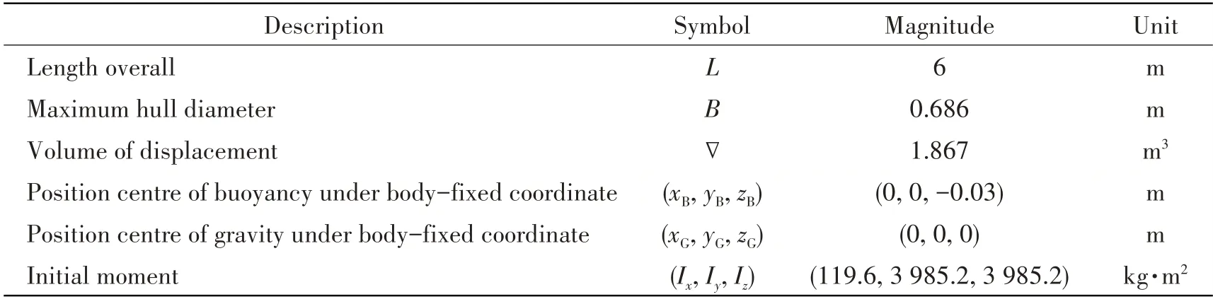
Tab.1 Main characteristics of the DRDC-STR submarine model

1.2 Coordinate system

For analyzing the motions of the submarine in 6 DOF,it is convenient to define two coordinate frames as indicated in Fig.2. The moving coordinate frameO-xyzis conveniently fixed to the submarine, namely the body-fixed reference frame. While the other is an Earth-fixed coordinate or an inertial coordinateE-ξηζwith the positive depthζpointing downwards.In the following,(ξ0,η0,ζ0)and(φ,θ,ψ)are the translation displacements and rotation angles of the object in Earth-fixed coordinate system. The definitions of linear velocity (u,v,w), angular velocity (p,q,r), external forces,and moments refer to the body-fixed coordinate.

Fig.2 Definition of coordinate systems

1.3 6 DOF module

The rigid model obeys Newton’s second law for submarine’s translational and rotation. The concrete equations of 6 DOF motion are shown in Eqs.(1)～(2).

whereFandMare the total force and moment acting on the submarine, respectively,B=(mu mv mw)is the momentum,K=(Ix p Iy q Iz r)is the moment of momentum,V=(u v w)is the submarine’s velocity,andΩ=(p q r)is the angular velocity.

2 Coefficient-based method

The coefficient-based model presented by Watt (2007)[3]is rewritten in this chapter. The forces and moments acting on the submarine can be described as functions of submarine state vectory=(u v w p q r ξ0η0ζ0φ θ ψ),as shown in Eq.(3).

whereXH,YH,ZH,KH,MHandNHrepresents the hydrodynamic loads acting on the hull of the submarine,XC,YC,ZC,KC,MCandNCrepresent the modeled control forces due to tail fin deflection,andXPandKPindicate propeller thrust and torque.

3 Direct CFD method

3.1 Governing equations and turbulence models

The Reynolds-averaged Navier-Stokes (RANS) equations are the governing equations to represent the kinematics and dynamics of viscous fluid, which are the kernel to calculate the 3-D viscous flow around the submarine in this paper.The specific form of RANS equations is shown as follows.

whereρ,μ,pandfiare the fluid density, viscosity coefficient, hydrostatic pressure and mass force per unit respectively;uiandujare the fluid velocity components; and the overbar (·) denotes timeaveraged components.

To close RANS equations, Wilcoxk-ωand SSTk-ωturbulence were chosen to solve for the viscous flow field around the submarine. The detailed derivation process and parameter selection can be found in the work by Larsson et al(2010)[12].

3.2 Mesh approach

Star-CCM+, which is a commercial CFD code, has provided many mesh discretization methods and the self-adapting trim mesh was chosen to perform calculations in present paper.The principle and concrete steps for the self-adapting trim mesh discretization can be seen in the reference written by Zhou et al (2017)[13]. Meanwhile, to resolve the viscous flow field around the submarine accurately, refinement grids were established in both submarine’s surface and near-field region withy+～1 to satisfy the turbulence model’s requirement. An overview of the computational meshes on the surface of the DRDC-STR model is shown in Fig.3. The computational region is cuboid-shaped with the size of 6.4L×3.4L×3.8Laround the submarine, whereLis the length of the submarine and the number of computed cells is about 328 million for the whole region.

Fig.3 Surface mesh discretization

The integral moving mesh was applied to simulate submarine 6-DOF motion. Compared with grid deformation and overset mesh algorithm, mesh reconfiguration and interpolations between subdomains can be avoided to guarantee the mesh’s quality and computational efficiency. During maneuvering motions, the calculation region moves or rotates with the mesh locked in a same position relative to the rigid submarine. Coupled with moving-mesh technology, boundary conditions for the cuboid region are composed of the following:The inlet is positioned 1.0Lupstream with an initial inflow velocity of 0 m/s while a pressure-outlet is positioned 2.0Ldownstream. Four remaining walls are set identical with the inlet,1.0Laway from the body.No-slip wall is set for the hull and appendages.

3.3 Validation of numerical method

For validation, straight-line towing simulations at different drift angles were performed for the DARPA Suboff model fitted with sail,stern rudders,ring wing,and four struts in an‘X’configuration,as illustrated in Fig.4.The experiment was carried out in the towing tank at NSWCCD and the data published by Roddy(1990)[14]can be used for validating CFD codes.

As shown in Fig.5,the predictions using the twok-ωmodels are in good agreement with experimental data with the drift angleβ＜12°.However,as the drift angle increases,the longitudinal force and heeling moment predictions by Wilcoxk-ωappear to match the measured data better than SSTk-ωpredictions.Although the vertical force and trimming moment calculated based on Wilcoxk-ωtend to over-predict with the drift angle 12°≤β≤16°,the tendency is similar compared with experiments.When the drift angle reaches 18°,the submarine’s hydrodynamic performance predicted by the two models deviates profusely from the experimental data,and the two models are not suitable for simulations with identical or larger attack angle. Based on above analysis, the Wilcoxk-ωwas chosen to simulate the submarine’s free-running maneuvers in the present paper.

Fig.4 Main particulars of full-appended Suboff model

Fig.5 Comparison of the submarine’s hydrodynamic performance between experimental and computational results

3.4 Calculation strategy

In this paper, the hydrodynamic loadsFHon the right-hand sides of the first six equations of Eq.(4) are evaluated by using URANS method seasonably. The hydrodynamic forces and moments acting on the submarine are evaluated by integrating pressure and shear data along the surface of the submarine.However,to reduce the complexity and computational requirements for direct CFD simulation, some coefficient-based models, as shown in Eqs.(5)～(6), are retained to account for the effect of propeller and control surface.The overall solution strategy for direct CFD simulation is presented in Fig.6.

Fig.6 Solution strategy

4 Results and discussions

Two typical maneuvers, including space spiral turning and vertical zigzag, were simulated based on methods presented in Chapters 3～4. The input rate of control surface deflection and straight sailing velocity were chosen as 3 °/s and 3 m/s for model cases, which indicated 0.878 °/s and 19.9 kn respectively for a full-scale submarine. The non-dimensional timetU0/Lwas chosen to describe motion histories,in whicht,U0andLrepresent time,straight sailing velocity and submarine’s overall length respectively. During these simulations, the self-propulsion state was first achieved before executing stern plane and rudder att=0 s.

4.1 Space spiral turning maneuver

Fig.7 Maneuvering strategy for space spiral motion

In this maneuver,the stern plane and rudder were executed at a constant rate to the desired angle att=0 s and then maintained throughout the maneuver. The time series of stern plane deflectionδsand rudder angleδrfor space spiral motion are shown in Fig.7 with the fixed values ofδs=-3°andδr=20°after the nondimensional timetU0/L=3.33.

The non-dimensional form of the linear velocity component (u，v，w) and angular velocity (p，q，r) versus non-dimensional time is shown in Fig.8. Quantitative agreement of non-dimensional ofu,qandrbased on the two approaches indicates that the current CFD method is reliable to a certain degree.Time histories ofpL/U0tend to fluctuate slightly during the steady turning strategy,while these changes did not appear in coefficient-based results.This phenomenon may be caused by unsteady flow,which is not easy to be modeled by maneuvering coefficients. Compared with the coefficient-based method,though the current CFD approach under-, and over-predicts the steady values ofvandwby about-19%and 23%respectively,these free-running trails show very similar tendencies versus time.

Fig.8 Time series of linear and angular velocities under body-fixed coordinate system

Fig.9 shows the evolution of roll and pitch as a function of non-dimensional time,and the horizontal projections of submarine’s trajectory were also depicted. This figure, at the beginning of the maneuver,when the maximum rudder rate is imposed,shows a roll and pitch excursion.The big distinction in pitch steady value from CFD and coefficient-based methods may be caused by submarine’s small longitudinal metacentric height and the difference in predicted trim hydrodynamics.As an important index to assess the submarine’s spiral turning ability, the tactical diameter of trajectory projections in the horizontal plane forecasted by CFD was about 1.07 times of the value from the coefficient-based method.

Fig.9 Roll,pitch and trajectory projections in horizontal plane

Fig.10 shows side views of submarine’s instantaneous representation in space spiral turning maneuver, and the vortical structures using iso-surfaces of the second invariant of the velocity gradient tensorQwere colored by velocity magnitude. Because the propeller is modeled by external force and torque, the acceleration and rotating effect acting on the flow field cannot be exhibited.Despite the simplicity of the propeller model, the tip vortex structures, which are produced by sail and stern planes,can also give a visualized maneuver process for analysis.

Fig.10 Side views of the submarine attached by iso-surface of Q=5 colored by velocity magnitude for spiral turning maneuver

The velocity field around the submarine during space spiral turning maneuver is shown at three representative transverse planes in Fig.11.The planes are taken around the submarine withx/L=0 (x-axis positive forward) being the position of the mid-ship. In this figure, the velocity magnitude details att=0 s(straight-ahead sailing),t=5 s(developing stage)andt=32.5 s(constant turning state) are represented. For the straight-ahead case, the velocity distribution shows good symmetry,and with the submarine entering into turning stage, the asymmetric velocity distribution caused by necklace vortices from the sail is significant. Moreover, the decrease of ship’s velocity for constant turning state can also be seen through contrasting these three cases.

Fig.11 Velocity field on different cross sections for submarine’s spiral turning maneuver(the x-axis origin placed at mid-ship)

4.2 Vertical zigzag maneuver

Theδs/θ=±5°/∓20°zigzag maneuver in vertical profile was also simulated using both the coefficient-based and direct CFD method.Before executing stern plane att=0 s, the self-propulsion was first achieved. Then the stern plane was deflected to 5°at a predetermined rate and kept at this state until the submarine’s pitch angle reached -20°,at which point the stern plane turned to-5°. Time series of the stern plane deflection and submarine’s pitch angle are shown in Fig.12,and six steering courses were conducted during the whole process.

The non-dimensional form of the linear velocity component (u,v,w)and angular velocity (p,q,r)are shown in Fig.13 and Fig.14,showing a good agreement either in value or tendency.Compared with the space spiral turning maneuver,less accumulated error may contribute to the more quantitative agreements of roll and pitch between the two methods.

Fig.12 Maneuvering strategy for vertical zigzag motion

Fig.13 Time series of linear and angular velocities under body-fixed coordinate system

Fig.14 Roll,pitch and translation in vertical direction

Fig.15 shows the flow field around the submarine in four states of P1,P2,P3and P4,whose positions are specifically illustrated in Fig.12.The hull of the boat is colored by pressure,while the slices are colored by vorticity to display flow revolution.The sail tip vortex developed from sail to stern is shown clearly, and tip vortices from the rudders made the submarine’s wake more complicated by coupling with inflow from the sail and the main-body.In addition,the differences of rudder pressure distribution are remarkable for these states, which were caused by larger attack angle in the tail region.

Fig.15 Vorticity field on different cross sections and pressure distribution on submarine’s surface

5 Concluding remarks

Direct CFD computations of a conventional submarine model undergoing space spiral turning and vertical zigzag maneuvers are presented. The integral moving mesh and URANS method coupled with 6 DOF kinematic module were chosen to model submarine’s 6 DOF motions. Through comparing the results from CFD approach and coefficient-based model,good agreement in time series of motion parameters indicates that the direct CFD method proposed in the present paper is an efficient and reliable tool for submarine maneuverability forecasting. Detailed flow physics can not only provide help for submarine’s maneuverability analysis but also suggest improvements to the coefficient-based model. Continuous improvements in faster parallel computers can offer more opportunities and foundations for direct CFD simulation of ship motions in the future.