A plotless density estimator with a Norton‑Rice distribution for ordered distances

Steen Magnussen

Abstract A Norton-Rice distribution (NRD) is a versatile,flexible distribution for k ordered distances from a random location to the k nearest objects. In a context of plotless density estimation (PDE) with n randomly chosen sample locations, and distances measured to the k = 6 nearest objects, the NRD provided a good fit to distance data from seven populations with a census of forest tree stem locations.More importantly, the three parameters of a NRD followed a simple trend with the order (1, …, 6) of observed distances.The trend is quantified and exploited in a proposed new PDE through a joint maximum likelihood estimation of the NRD parameters expressed as a functions of distance order. In simulated probability sampling from the seven populations,the proposed PDE had the lowest overall bias with a good performance potential when compared to three alternative PDEs. However, absolute bias increased by 0.8 percentage points when sample size decreased from 20 to 10. In terms of root mean squared error (RMSE), the new proposed estimator was at par with an estimator published in Ecology when this study was wrapping up, but otherwise superior to the remaining two investigated PDEs. Coverage of nominal 95% confidence intervals averaged 0.94 for the new proposed estimators and 0.90, 0.96, and 0.90 for the comparison PDEs. Despite tangible improvements in PDEs over the last decades, a globally least biased PDE remains elusive.

Keywords Fixed-count sampling · Spatial point pattern ·Distance distributions · Forest inventory · Joint maximum likelihood estimation · Bias · Root mean squared error ·Coverage

Introduction

Fixed count or plotless sampling designs have a long history in both ecology and forestry (Shanks 1954; Prodan 1968;Mark and Esler 1970; Lynch and Rusydi 1999; Cogbill et al. 2018). In ecology, the objective is typically directed towards gaining information about diversity, spatial distribution, and the density of various objects of interest (Chen and Tsai 1980; Clayton and Cox 1986; Coddington et al. 1991;Barbour and Gerritsen 1996). In forestry, applications may also target population parameters such as volume, stem size,height, and basal area in stands defined by species, canopy structures, and age (Kleinn and Vilčko 2006; Staupendahl 2008; Haxtema et al. 2012; Magnussen 2016). For both types of applications, new developments to curtail bias and reduce sensitivity to spatial point patterns continue to this day (Magnussen 2016; Ott and Errico 2016; Ducey 2018;Sohrabi 2018; Shen et al. 2020) providing users with a growing list of plotless density estimators (PDEs) to consider.The a priori fixation of the sampling effort—in terms of the number of objects (k) to sample at a sample location—is the feature that renders PDEs design-biased (Chambers 2011). A design-unbiased PDE withkdetermined locally is possible but also impractical (Fehrmann et al. 2011; Ott and Errico 2016).

A PDE can only aspire to be model-unbiased if the spatial point pattern matches the point pattern assumed for a modelbased estimator (Eberhardt 1967; Pollard 1971; Picard et al.2005; Shen et al. 2020). As a rule, bias decreases with an increase ink(Kleinn and Vilčko 2006; Kronenfeld 2009;Ramezani et al. 2016). Several studies have suggested that bias with ak-value of 6 can be less than 6% in applications with estimators developed in the last few decades (Prodan 1968; Staupendahl 2008; Kronenfeld 2009; Fleiss et al.2013; Magnussen 2016) or by serendipity (Ramezani et al.2016; Jamali et al. 2020) with a simple ‘basic’ estimator first proposed by Moore (1954) and later—with theoretical underpinnings—by Eberhardt (1967). The bias of a PDE can even be as low as 1‒3% which makes PDEs—in terms of efficiency—competitive with fixed area sampling (Lessard et al. 2002; Magnussen 2014; Safari et al. 2020), but only in populations with a moderate degree of clustering or overdispersion. A valid inference about the spatial distribution of objects in a population fromn×kobserved distances is,however, only possible for impractically large sample sizes(Diggle 1983; Cressie and Collins 2001; Møller and Waagepetersen 2004; Illian et al. 2008).

If we consider the intrinsic bias from fixingkas unresolvable from a standpoint of theory, improvements in PDEs are possible with a distance distribution that accommodates the widest spectra of spatial point patterns, and from a better use of the collected distance data. In just about all PDEs, only the distance to thekth object is used. One exception is the PDE proposed by Kleinn and Vilčko (2006) in which the distances to thekth and (k+ 1)th nearest object were combined.Another is the use of the density in the annuli defined by the firstk−1 distances, and a regression approach to predict the density in thekth annulus (Magnussen et al. 2008). A PDE building on the information contained in the distribution ofkordered distances from each ofnsample locations may be less sensitive to the spatial point pattern in a population.Fork= 6, the sensitivity of PDEs to the spatial point pattern appears to be the biggest obstacle to progress and wider use.

The use ofn×kobserved and ordered distances will only be efficient with a single distribution function, and trends in the parameters of this distribution that are consistent with observed trends in either raw or central moments of ordered distances (Pollard 1971; Stoyan et al. 2001).

This study identifies the Norton-Rice distribution NRD by Norton et al. (1955) as a distribution that affords the simultaneous use of alln×kobserved distances for the purpose of constructing an otherwise conventional PDE (see, Picard et al. 2005, for an overview) with no attempt to address the bias issue beyond the discount of thekth object as proposed by Moore (1954) and Eberhardt (1967). The performance of the proposed new PDE is compared to the performance of three alternative PDEs, two selected based on an expected strong performance, and one (the Moore–Eberhardt) based on its practical appeal of simplicity. Simulated fixed-count sampling, withk= 6 from seven populations with known locations of forest trees, three sample sizes, and 1200 replications is the basis for the performance assessment.

The study demonstrates the suitability of the NRD, and the good (robust) performance of the proposed PDE and points to further improvements with larger sample sizes that afford estimation of a joint multivariate distribution for ordered distances.

Materials and methods

This section begins with results supporting the choice of an RND as a suitable distribution for the distancesrijfrom theith sample location (i= 1, …,n) to thejth nearest object(j= 1, …,k) with parameters (mj,aj,bj) that can be expressed as simple functions ofjso that a PDE constructed from a RND uses all the information collected in then×kdistances.A section then follows with definitions of the new proposed PDE, three alternative PDEs, and a benchmark estimator for fixed area sampling with circular plots (Schreuder et al.1993). The last four sections deal with: (1) a brief step-bystep guide to practical applications with the proposed PDE;(2) the performance criteria for the assessment of the new PDE; (3) simulated probability sampling; and (4) data from seven stem maps of forest tree locations.

A suitable distribution function for rij

The search began with 13 candidate distributions with a domain of support restricted to R+. They are: the Beckmann-, the Chi-square-, the Frechet-, the Gamma-, the Inverse-Gaussian-, the Levy-, the Log-normal-, the Maxwell-, the Negative Binomial-, the Norton-Rice-, the Rayleigh-, the Rice-, and the Weibull-distribution. Of these,only the Beckmann and the Norton-Rice, the Rayleigh, and the Rice distributions are designed for the distribution of the norm of a vector in a 2D space (Norton et al. 1955;Gupta and Song 1997; Zhu et al. 2017). The Beckmann distribution was fitted under the assumption that: (1) the coordinates (x,y) of an object location are uncorrelated;(2) the means in the presumed bivariate normal distribution of object location coordinates are equal and zero when centered on a sample location; and, (3) the standard deviation in centered object coordinates is equal in both cardinal directions. For the largest sample size in this study (20),the assumptions were supported by appropriate hypothesis tests. With Holm’s sequential rejection test (Holm 1979),the rejection rate of the null hypothesis was in all cases less than 0.05. When fitting a Norton-Rice distribution to data, it is important to start the iterative fitting algorithm from reasonable initial guesses of the parameter values(Koay and Basser 2006). Form, we used the value of 1,foraandb, we used the maximum likelihood value of the standard deviation from the fitted Beckmann distribution.These starting values are sensible because a Beckmann distribution is a special case of the more general Norton-Rice distribution. If we let the algorithm select its own starting values, the desired trend in the parameters across distance orders would have become obscure.

For the data and sampling designs in this study (c.f.sections on sampling designs and data), a three-parameter Weibull distribution most often achieved the best fit to individual data sets ofndistances to thejth nearest object(Criterion: BIC, Raftery 1999). It was closely followed—in order of average BIC—by the two-parameter gamma distribution, the Norton-Rice, and the Rice distributions.All differences in terms of average BIC-values in this group of four distributions were less than 3. On average over the 1200 replications for a site, the difference between the best and fourth ranked distribution varied from ‒ 0.21 to ‒ 0.57 or 2% to 5% on a relative scale. The Negative-Binomial distribution never made it to the top four; its highest rank was seven. This ‘poor’ performance was a surprise (cf., Gao 2013) since the parameter to be estimated is the desired density (Eberhardt 1967), but Eberhardt does admonish against using this distribution when the density is unknown.

Only the maximum likelihood estimates (MLEs) of the three parameters of a Norton-Rice and the single parameter of standard deviation in a Beckmann distribution displayed a simple trend with the orderjof observed distances (j= 1, …,k= 6). The choice between the Norton-Rice and the Beckmann distribution was decided by two additional goodness of fit tests. The first was a locationt-test of equal means(sample mean versus predicted mean), and the second was a test of equal variance in sample observations of distances of orderj(j= 1, …,k= 6), and in predicted distances from a fitted distribution (Levene 1960). The Norton-Rice distribution passed these tests with no rejection of the null hypotheses at the 5% level (adjusted for multiple tests with Holm’s sequential rejection test (Holm 1979)). The Beckmann distribution also passed the test of equal means without any rejections of the null hypotheses, but in three of the seven populations,there was a high rate of rejections (> 0.25) in the test of equal variance. In conclusion: the Norton-Rice distribution was chosen as a suitable distribution of distances for the purpose of defining a PDE which uses information from alln×kobserved distances.

To summarize the goodness of fit for the NRD: in a total of 7 (populations) × 6 (distances) × 3 (sample sizes) × 1200(replications) or 151,200 tests, the rate of rejection of the hypothesis with Holm’s sequential rejection test applied to data from one population, one distance, and one sample size was zero for: (1) the tests of equality in distribution(Anderson–Darling test, Anderson and Darling (1952)),(2) equal means (t-test), and (3) equal variances (Levene 1960).

Randomly chosen examples with one sample size(n= 20) illustrate in Figs. 1, 2, and 3—in the form of probability plots—the goodness-of-fit attained with a RND.

Since the RND is, in general, not well known, its probability density function (f) is provided:

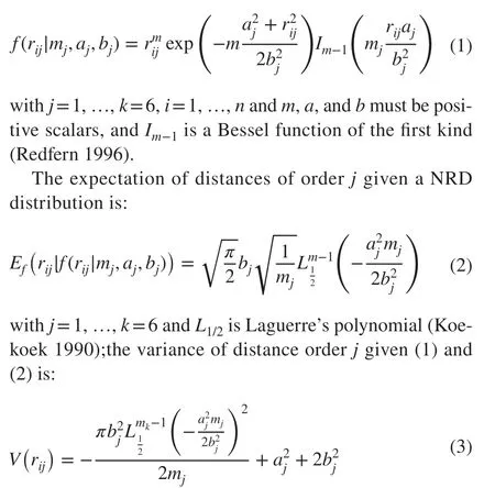
withj= 1, …,k= 6. Expressions for the skewness and kurtosis are in the "Appendix"; they are, however, exceedingly complex. Suffice to say that skewness of the NRD can vary from 0 to approximately 8, and kurtosis from 0 to approximately 100. A negative skewness is impossible, but also not relevant for the distribution of distances as they are a monotone function of squared projected distances in two cardinal directions. The tails of the NRD are much thinner than in any of the other investigated distributions. In an ecological context, and sampling from a finite population of objects,the exponential thinning of tail probabilities minimizes the potential of otherwise inconsistent crossings of distribution functions for distance ordersj= 1, …,k= 6.

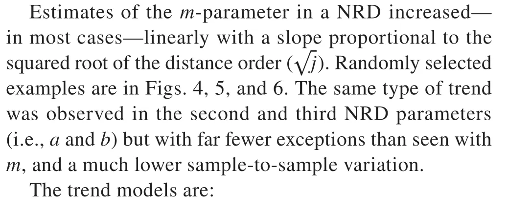
Fig. 1 A probability plot indicating the fit of a Norton-Rice distribution to n = 20 observed distances from each distance order j = 1, …, k = 6 in a randomly chosen replication (368)from the Lansing population

It should be emphasized that a joint estimation of the RND parameters does not result in ak-dimensional multivariate distribution but merelyklinked marginal distributions. Fixed-count distance data does not afford a direct estimation of a joint distribution due to the ordering imposed on recorded distances, and the stopping rule dictated by the choice ofk. Equally, ak-variate orderdistribution (Sarhan and Greenberg 1962) is unattainable,as the underlying unrestricted distribution of the distance from a random sample location to a randomly selected object remains unknown.

Estimators of density

The proposed new PDE belongs to the first-order moment estimator of density (Morisita 1954; Cottam and Curtis 1956; Persson 1964; Byth 1982) that uses the square ofthe expected value of the inverse distance of orderk. The new estimator is defined in (5). In the cited references, the expected value was taken as the sample mean of inverse distances. For the proposed PDE, the expectation is computed as the mean over an assumed RND distribution with parameters obtained from (4) with least squares estimates of the regression parameters and settingj= 1, …,k= 6.This type of PDE has been bestowed robust properties by the cited authors and others:

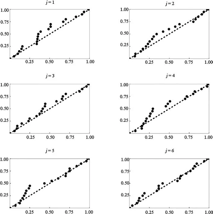
Fig. 2 A probability plot indicating the fit of a Norton-Rice distribution to n = 20 observed distances from each distance order j = 1, …, k = 6 in a randomly chosen replication (950)from the Ponderosa population

However, this estimator is very unstable due to the integration over squared distances close to zero. Instead a bootstrap estimator of variance (Efron and Tibshirani 1993) is recommended. Specifically:

The first alternative PDE is due to Shen et al. (2020)and published inEcologywhen this study was finishing. It is given in (8). Their estimator is derived analytically from the distribution of ordered distances in a population where the spatial distribution of the number of objects per unit area follows a negative binomial distribution (NBD) (Gao 2013). The strong performance of this novel type of PDEestimator as documented by Shen et al. (2020) motivated inclusion in this study:

Fig. 3 A probability plot indicating the fit of a Norton-Rice distribution to n = 20 observed distances from each distance order j = 1, …, k = 6 in a randomly chosen replication (620)from the regular population

Fig. 4 Trends in the Norton-Norton distribution parameters m (top),a (middle) and b (bottom) in 20 randomly selected replications from population Tall pines (gray lines). Full line is the least squares trend line over distance order j = 1, …, k = 6. Black dashed lines represent a 95% confidence interval for a prediction of a parameter value given j and n = 20

The authors did not provide an estimator of variance.Here we again resort to a bootstrap variance estimator, also withB= 100.

The second alternative PDE is in (9). It was proposed by the author as a robust estimator with moderate levels of bias when tested in 27 forest stands with a census of tree locations(Magnussen 2015):

Fig. 5 Trends in the Norton-Norton distribution parameters m (top),a (middle) and b (bottom) in 20 randomly selected replications from population Lansing (gray lines). Full line is the least squares trend line over distance order j = 1, …, k = 6. Black dashed lines represent a 95% confidence interval for a prediction of a parameter value given j and n = 20

Fig. 6 Trends in the Norton-Rice distribution parameters m (top), a(middle) and b (bottom) in 20 randomly selected replications from population Paracou (gray lines). Full line is the least squares trend line over distance order j, j = 1, …, k = 6. Black dashed lines represent a 95% confidence interval for a prediction of a parameter value given j and n = 20

Fig. 7 A randomly selected example (rep. 910) from Lansing of jointly fitted RNDs for distance orders 1, …, 6, 7, and 8, whereby the last two are predictions for non-observed distance orders

Fig. 8 A randomly selected example from Paracou (rep. 281) of jointly fitted RNDs for distance orders 1, …, 6, 7, and 8, whereby the last two are predictions for non-observed distance orders

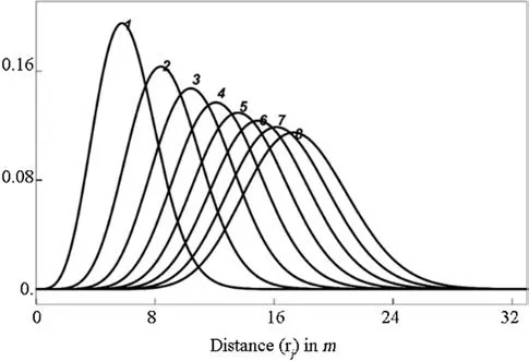
Fig. 9 A randomly selected example from regular (rep. 227) of jointly fitted RNDs for distance orders 1, …, 6, 7, and 8, whereby the last two are predictions for non-observed distance orders

The last alternative PDE was first introduced by Moore(1954) and later by (Eberhardt 1967). It is popular due to both simplicity and good performance in several studies where the spatial point pattern of object locations displays no more than a weak clustering or a weak overdispersion(Lessard et al. 2002; Kleinn and Vilčko 2006; Haxtema et al. 2012; Ramezani et al. 2016). It is, however, an estimator that employs squared inverse distances which can generate a serious bias in clustered point patterns(Steinke and Hennenberg 2006; Staupendahl 2008). The Moore–Eberhardt estimator is:

Application guide

Users who wish to use the new PDE(k) in (5) can do so by following these steps:

1. Fit by MLE the three parametersm,a, andbin an RND to eachksets ofndistance data of orderj= 1, …,kwithk≥ 3.

2. Obtain, by least squares, the regression parameters in(4) to capture the trends inm,a, andbacross orders of distance.

Performance criteria

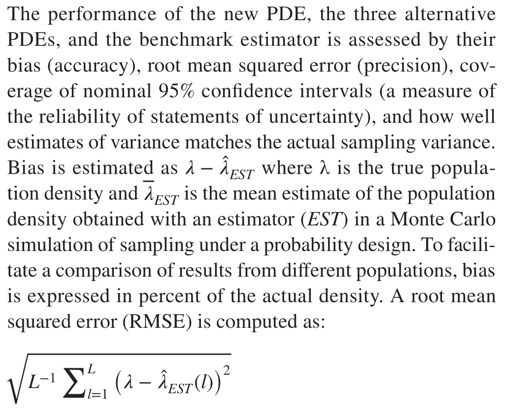
where(l) is thelth ofLindependent estimates of the population density λ obtained with an estimatorEST. Again,RMSE is expressed in percent of λ. Coverage of a nominal 95% confidence interval for the actual density was computed as the fraction ofLpredicted intervals that include the actual density. In thelth replication and for a sample sizen, a nominal 95% confidence interval forλwas computed as the closed interval:

wheretn‒1,0.975is the 97.5 percentile in Student’st-distribution withn−1 degrees of freedom.

Simulated sampling

Estimates of population densities, variances, and confidence intervals were obtained with replicated simulated probability sampling in seven populations (see next section on data).

For the four PDEs, the value ofkwas fixed at 6. Hence,at each ofnrandomly selected sample locations in a population, the distance in meters to the six nearest objects (here:trees) is measured and recorded (i.e.,rij,i= 1, …,n,j= 1,…,k) to allow estimation of density and variance as per Eqs. (5) to (12). The benchmark estimator of density at theith sample location was obtained from counting the objects within a fixed area circular plot with areaA, and dividing this byA. At the completion ofnsample locations, the estimate of the population density and variance is obtained from(13) and (14).

Three sample sizes of 10, 15, and 20 are used in this study, and three plot sizes with areaAof 200, 300, and 400 m2is used with the benchmark estimator. Each round of probability sampling and estimation was replicatedL= 1200 times to allow stable estimates of bias, RMSE, coverage, and agreement between the Monte Carlo sampling variance in 1200 estimates of density and the average analytical estimate of variance.

Sample locations were in each population (see next)determined in a two-stage process. In stage I, a set ofntriangles out of 40 were selected at random with probability proportional to size and without replacement; in stage II, a sample location was chosen at random within each selected triangle. The 40 triangles would completely tessellate a population and efforts were made to ensure triangles of approximately equal size. The sample location selection was designed to emulate a non-aligned systematic sampling with the benefit of an approximately uniform sampling intensity across the space of a population (Ripley 1988). The estimators presented in (5) to (14) assumes an equal probability sampling.

To minimize edge effects, when a sample location was closer to the edge than one of the distancesrijor a fixed area plot radius, a ‘mirage’ corrections was implemented as proposed for PDEs by Lynch (2012), and for fixed area sampling by Gregoire and Scott (2003).

Data

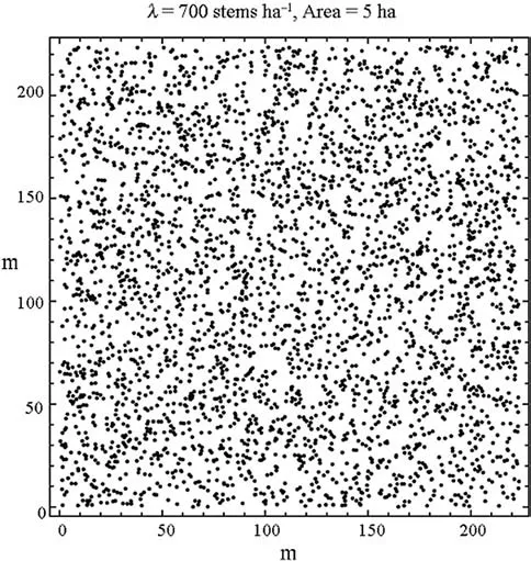
Fig. 10 The csr700 population of 3500 stem locations. The locations are a realization of a completely random spatial process (c.s.r.) (Ripley 1988)

Fig. 11 The Tall pines population of tree locations

Data in the form of forest tree locations (x,y) from seven populations are used in this study. The first population constitutes a simulation of a complete spatial random distribution of 3,500 locations within a 5.0 ha area in the form of a square. Accordingly, the density is 700 stems per ha, or 0.07 per m2; the population is calledcsr700(Fig. 10).

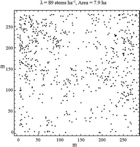
Fig. 12 The Lansing population of tree locations

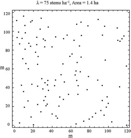
Fig. 13 The Ponderosa population of tree locations

The second data set (population) is calledTall pinesand comes from the Tallahassee Research Station in Wade County Florida (Platt et al. 1988).Tall pinesare known to exhibit clustering at multiple scales (Stoyan 2000). A map of 584 stem locations in a 4-ha area is in Fig. 11.

The third data set,Lansing, is from an investigation in a 281.6 m × 281.6 m (7.9 ha) mixed hardwoods plot in Lansing, Clinton County, Michigan USA (Gerrard 1969) with 703 tree locations (density is 89 stems per ha). A map of tree locations is in Fig. 12.

The fourth data set,Ponderosa, constitutes the locations of 108 Ponderosa pines in a 120 m square plot (1.44 ha) in the Klamath National Forest in northern California, published as Fig. 2 in Getis and Ord (1992). Accordingly, the density is 75 stems per ha (Fig. 13). The fifth data set, Paracou, is composed of the locations of 675 adult and juvenile Kimboto trees (Pradosia cochlearia or P. ptychandra) in a square 400 m × 400 m (16 ha) plot near Paracou in French Guiana (Flores 2005). The density is 42 stems per ha; a stem map is in Fig. 14. The sixth data set, BCI, is composed of 3,444 locations of trees in the genus salicaceae in a 100 m× 500 m area (5 ha) with a density of 69 stems per ha in the Barro Colorado Island research plot in Panama (Condit and Hubbell 1998). A stem map is in Fig. 15. The last data set,regular, was generated from a regular 10 m ×10 m grid of tree locations in a square 5.0 ha area that were relocated by a random direction (0 to 2 π) and a random displacement between 0 and 4 m. The locations of 401 stems remaining within this area (i.e. density is 80 stems per ha) are shown in Fig. 16.

Data sets two to six were downloaded in May 2020 from the R-packagespatstat(https:// cran.r- proje ct. org/ web/ packa ges/ spats tat, Baddeley et al. (2015)).

Population summaries of the mean, variance, skewness,and kurtosis of distances from a random sample location to the nearest, the third nearest, and the sixth nearest stem location are in Table 1. To note is the increase in variance of distances to the nearest, third nearest, and sixth nearest stem location and a considerable among-population variation in this increase. Within each population, both skewness and kurtosis of ordered distances decrease along a monotone gradient from the nearest to the sixth nearest stem location.

Results

Bias

Over the seven populations and three sample sizes, the average percent bias of the population specific stem density was‒ 0.6% forλNRD, ‒ 1.8% forλNBD, 5.8% forλS, and ‒ 8.8%forλME. The overall bias forλNRDwas significantly (t-test,p< 0.01) less than with any of the alternative PDEs but also significantly greater than the average relative bias of 0.3%withλFIXand a plot size of 200 m2. On aperpopulation basis, the relative bias ofλRNDwas significantly the lowest inTall pines(‒ 1.1%),Paracou(1.5%),BCI(‒ 2.9%), andregular(0.0%). Incsr700,LansingandPonderosa, the least biased estimator wasλNBDwith averages of ‒ 0.9%, ‒ 0.6%,and 0.0%, respectively. The among-population variation in bias was forn= 20 andn= 10, lowest forλNRD, second lowest forλNBD, and highest forλME(Table 2). Density estimates withλRNDwere strongly correlated with estimates obtained withλNBD(0.94). The performance ofλSandλMEwas the most variable, and with a poor performance (bias > 9%) in three (λS) and two populations (λME). Sample size did not appear to influence the estimate of relative bias inλNBD,λS,orλME. InλNRD, however, bias drifted from 0.6% withn= 20 to ‒ 2.1% withn= 10.

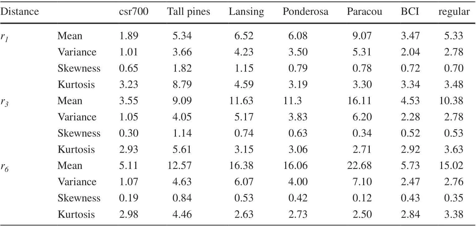
Table 1 Population summary statistics of the distance r (unit:m) from a random sample location to the nearest (r1), third nearest (r3) and sixth nearest(r6) tree

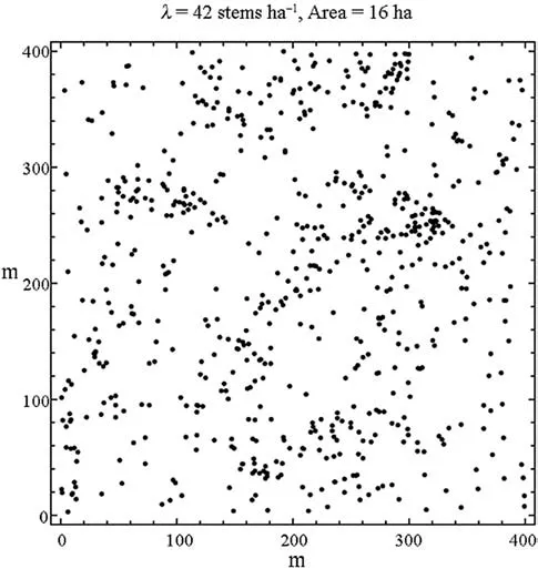
Fig. 14 The Paracou population of tree locations

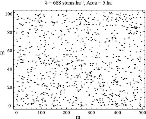
Fig. 15 The BCI population of stem locations of trees in the Salicaceae family

Root mean squared error

Root mean squared error in percent of the population stem density (RMSE%) was on average, (over populations and sample sizes), 13% forλRNDandλNBD, and 14% for, andλME. A bootstrap estimate of 1.1% for the standard error in these estimates suggests that they were equal. Individual estimates are in Table 3. When averaged over sample sizes,a difference of approximately 2% would be declared significant at the 0.05 level or less. Accordingly, significant differences among the RMSEs of the PDEs were limited to populationsLansingandBCI. InLansing, the RMSE% ofλSwas 18% and significantly greater than the 14% reported forλRND,λNBD, andλME. InBCI,the RMSE% ofλME(27%)was significantly greater than the RMSE% of the remaining three PDEs, and the RMSE% ofλSwas 18% significantly less than the RMSE of any other estimator. RMSE% ofλRNDandλNBDinBCIwas 21% and significantly greater than the RMSE% ofλSbut also significantly less than the RMSE%ofλME. A reduction in sample size from 20 to 10 increased the RMSE% between 20 and 70%. Stochastic variation in the estimates of bias is regarded as the main reason why the expected increase of 40% for an unbiased estimator was not attained.

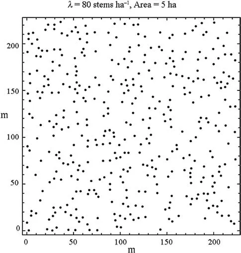
Fig. 16 The regular population of stem locations

Table 2 Bias in percent of actual population stem density

Table 3 Root mean squared errors in percent of the actual population stem density

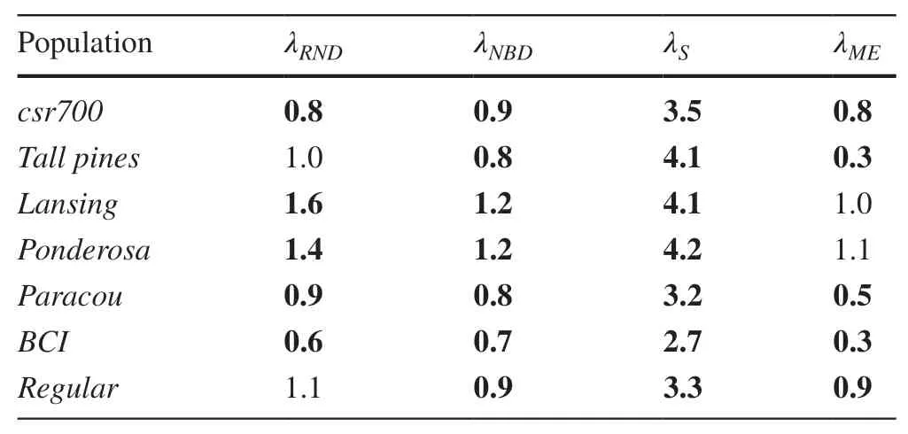
Table 4 Ratios of the average of analytical variance estimates to the variance of the 1,200 estimates of stem density

With fixed area sampling, the overall average RMSE%was 11% with 400 m2plots, 13% with 300 m2plots, and 14%with 200 m2plots. If calibrated to a sample yield ofk= 6 trees per plot, the sampling with fixed area plots generates an RMSE% that is approximately 20% lower than attainable with the PDEsλNRD,λNBD, andλS, and approximately 30%lower than withλME.

Analytical and empirical estimates of variance

The estimators of variance in a PDE should indicate, for a given sample size, the expected variance in repeated sampling under a given sampling design. The ratio of the mean analytical estimate of variance (taken over the 1200 replications of a sampling design) to the variance of the 1200 estimates of variance captures how well the analytical variance predicts an unbiased estimate of the variance due to sampling. With a sample size of 20, the average ratio was 1.06 forλNRD, 0.91 forλNBD, 3.6 forλSand 0.7 forλME.(Table 4). These ratios would increase by approximately 30% when the sample size was 10. Sampling with fixed area plots produced the least variable ratios, with a range(n= 20) from 1.0 to 1.3 with the lowest ratios observed with the largest plot size.

Table 5 Coverage of nominal 95% confidence intervals for λ

Coverage

Over all populations and sample sizes, the coverage was 0.96 (range 0.88‒1.00) forλNRD, 0.92 (range 0.86‒0.96)forλNBD, 0.97 (range 0.92‒1.00) forλS, and 0.92 (range 0.88‒0.96) forλME.Coverage was, for all four PDEs, as a rule, significantly different from the target of 0.95.

Coverage decreased by an average of 0.04 with a decrease in sample size from 20 to 10 with only minor differences among the four PDEs. The coverage ofλNRDwas moderately correlated (0.7‒0.8 after a transformation to arc tan) with the coverage ofλNBD,λS, andλME.The only strong correlation (0.96) was betweenλNBDandλME..Detailed results are in Table 5.

With fixed area plots, the coverage was an average of 0.94 (range 0.88‒0.98) for all three plot-sizes, and the among-population variation for a given sample size was considerably less than with any of the PDEs. Coverage also decreased with sample size, but only by 0.03 when sample size decreased from 20 to 10. The minimum coverage was 0.89 inParacouwithn= 10.

Discussion and conclusions

The new proposed estimator, like others proposed by the author (Magnussen et al. 2008, 2011; Magnussen 2012a,2012b, 2014, 2015) appears to be both robust and with an attractive performance within the class of PDEs. Yet it also requires complex computations that, apparently, have been an obstacle to uptake in both forestry and ecology where simpler and typically more biased and less precise PDEs are still popular (Ramezani et al. 2016; Cogbill et al. 2018;Sohrabi 2018; Jamali et al. 2020; Safari et al. 2020). If the proposed new PDE had been computed only from the squared mean of theninversekth-order distances (Cottam and Curtis 1956; Cogbill et al. 2018), the performance would have been no better than the performance of the Moore–Eberhardt estimator (ME). An attempt was also made to improve—in the same way as done for the proposed new PDE—the type of basic PDEs that uses the inverse of the mean of squared distances (for examples, Morisita 1954; Kendall and Moran 1963; Pollard 1971), but the attempt failed inasmuch as performance deterioratedvis-à-visthe original PDE. For this type of PDEs, the use of the inverse of the squared mean ofn kth order distances plus their variance seems to be a better strategy (Pollard 1971; Magnussen 2016).

Using the full information about alln×kdistances collected in a sample lessened an otherwise marked dependency betweenkand performance (Kleinn and Vilčko 2006; Kronenfeld 2009; Haxtema et al. 2012). The performance of the proposed estimator was virtually identical fork= 4, 5, and 6(not shown), and for predictions of 7th and 8th order distances.Thus, it may be advantageous for a fixed sampling budget to increase the sample size and lowerkfrom a preferred value of,say, six to five or even four (Steinke and Hennenberg 2006).

The full potential of using the NRD for modelling thekordered distances was not exploited in this study. A joint multivariate distribution would be required to simulate sampling with virtual fixed area plots (Magnussen 2012a), or for emulating a fixed area plot by computing the probability integral of having exactlyktrees within a given distance from a random sample location (Pollard 1971). Sample sizes of 10, 15,and 20 are too small to afford a reliable estimation of a correlation matrix fork= 6 ordered distances (Chen et al. 2006)which would be needed to tie thekjointly fitted marginal distributions into a multivariate distribution via a copula (Fischer 2010). For PDE in a large population where sample sizes can be in excess of 100 (Shen et al. 2020), a density estimator based on ak-variate joint NRD may prove worthwhile.

The proposed new PDE is at least at par with the attractive PDE published by Shen et al. (2020) inEcologywhen this study was coming to an end. Their PDE is admittedly much simpler and easier to implement than the one proposed here.The estimator by Shen et al. (2020) could not be improved upon by assuming an RND for thekth order distances. With its relative simple structure, the Shen et al. (2020) PDE has,admittedly, a much greater chance to become popular both in forestry and ecology even if computational complexity ought not to deter usage of an otherwise robust and attractive PDE when excellent computational resources and the technical support for implementation of a more complex PDE are available.

The robustness referred to here is with respect to the performance across a set of seven populations. In practical implementation of a PDE, an estimator with a low sensitivity to measurement errors is desirable. In plotless sampling,measurement errors are typically linked to the rank of an associated distance measurement. In dense forests, and when sampling for rare species, it is not uncommon that a field crew misses a tree in the search for thekth nearest tree to a sample location. How are the results—with the proposed PDE, and the three comparison PDEs—affected by this kind of error? To get an idea, a small simulation study was done in which 10% of the samples were in error. To limit the scope of this investigation, only a sample size of 20 was considered.The error was simulated as a skipped (undetected) tree. Thus,in 10% of the samples, the presumed distance to the sixth tree was in effect the distance to the 7th tree. Consequently,the measurement errors lead to a decrease in the estimates of stem density. With the proposed PDE, the decline was nearly 1.0% on all sites with a minor (0.2%) decrease also in the empirical standard deviation of the 1,200 collected estimates of density. With the estimator proposed by Shen et al. (2020), the density estimates changed by 1.5% with a concomitant decrease in the among-replicate standard deviation of 1.5%. Finally, estimates obtained with theandestimators dropped by 1.5% to 3.3% (mean = 1.9%),also with a reduction in the among-replicate standard deviation of 0.2% on all sites. The decline in standard deviations is explained by inverse distances in the estimator. Given that a PDE, when applied in a single population, can deliver estimates with either a positive or a negative bias, it is not possible to draw strong conclusions from this investigation of robustness against measurement errors apart from saying that the Moore-Eberhard estimator appears to be the least ‘robust’and that the proposed new estimator holds a narrow edge over the estimator proposed by Shen et al. (2020).

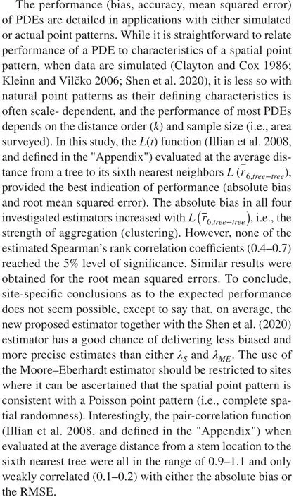
Modelling of ordered distances with the RND can also facilitate simulations of spatial point patterns based on data collected in fixed-count sampling (Nothdurft et al. 2010), in particular when equipped with an angular distribution function (Rose 1953) to capture departures from a uniform distribution. The high RMSEs inBCIcan be attributed, in part,to a highly significant angular correlation of 0.68 between distances of order five and six. In no other population did the absolute angular correlation exceed 0.07.

Appendix

The mean (location) and variance of a Norton-Rice distribution (cf (1)) with parameters {mij, aij, bij} at theith site andjth distance are given in (2) and (3). For the sake of completeness, the expressions for the skewness coefficient and the kurtosis is given next.

The skewness coefficient of a RND can be computed from the three parameters as per (15) with subscripts dropped for clarity.

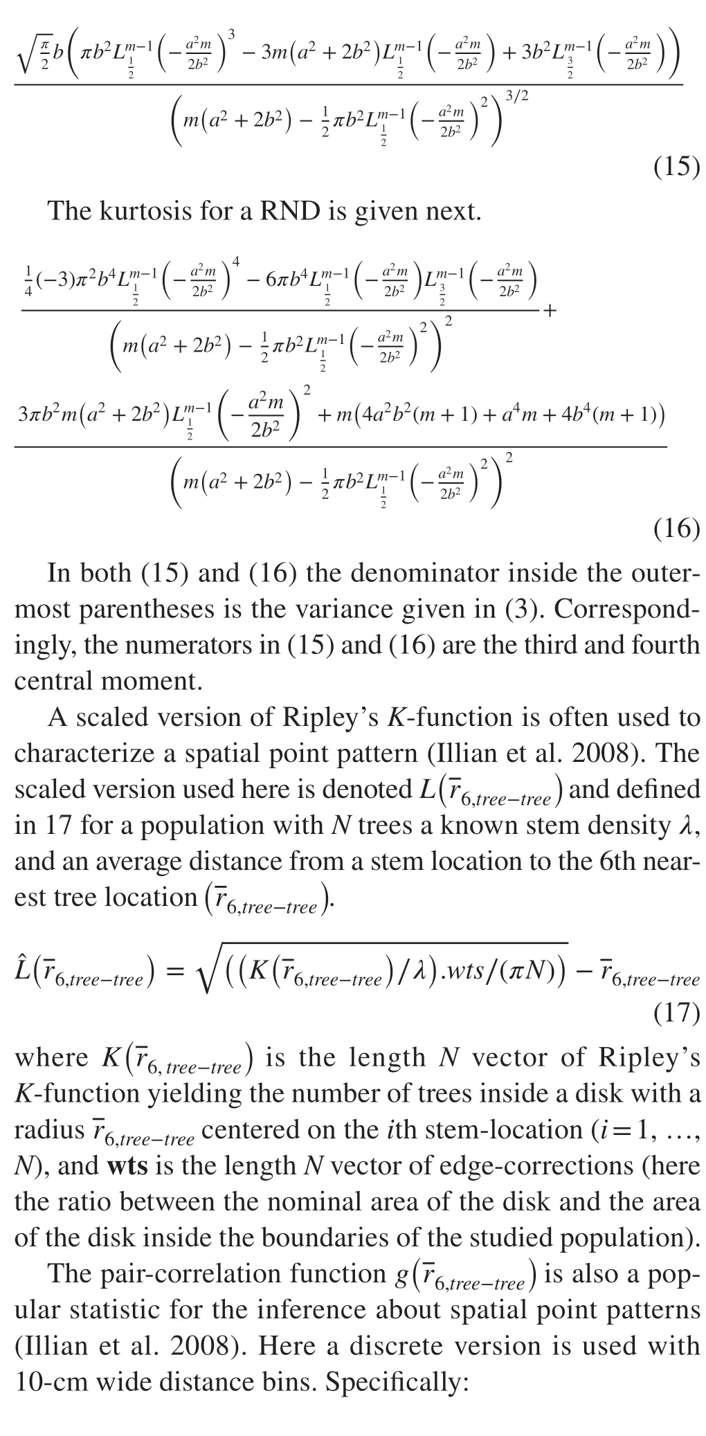
whererijis the distance from theith tree to thejth treej≠i=1,…,Nin the population. To minimize edge effects,the boundary mirage by Lynch (Ibid) was used.