The North Equatorial Current/Undercurrent volume transport and its 40-day variability from a mooring array along 130°E*

Xin YUAN , Qingye WANG , Junqiao FENG , Dunxin HU

1 Key Laboratory of Ocean Circulation and Waves, Institute of Oceanology, Chinese Academy of Sciences, Qingdao 266071,China

2 University of Chinese Academy of Sciences, Beijing 100049, China

3 Center for Ocean Mega-Science, Chinese Academy of Sciences, Qingdao 266071, China

4 Laboratory for Ocean and Climate Dynamics, Pilot National Laboratory for Marine Science and Technology (Qingdao),Qingdao 266237, China

Abstract Traditionally, the estimated volume transport of the North Equatorial Current/Undercurrent(NEC/NEUC) is based on geostrophic equations and/or model results; however, direct observational evidence has not been acquired. We focused on one-year mooring observation data collected along 130°E and calculated the NEC/NEUC volume transport and explore its variability. Results show that the mean NEC and NEUC volume transports calculated from the mean velocity structures in the upper 950 m are 39 Sv and 6 Sv, respectively. Analysis of daily mooring data indicated that the volume transport of the NEC is approximately 52 (±14) Sv and the volume transport of the NEUC is approximately 18 (±13) Sv.A signif icant 40-day variation existed for the volume transport of both the NEC and NEUC. Overall, the intraseasonal variability of the NEC is vertically coherent with that of the NEUC. Observations indicated that the NEUC has three cores centered at approximately 8.5°N (～500 m), 12.5°N (～700 m), and 17.5°N(～900 m), of which the middle core (12.5°N) is the strongest. The 40-day variability of the NEC and NEUC is related to the variability of local wind stress curl anomalies among various Madden-Julian Oscillation phases. When local wind f ield generates a negative (positive) wind stress curl anomaly, a weaker NEC(NEUC) and stronger NEUC (NEC) would occur.

Keyword: intraseasonal variability (ISV); North Equatorial Current/Undercurrent (NEC/NEUC); transport;Madden-Julian Oscillation (MJO)

1 INTRODUCTION

The circulation system of the Western Tropical Pacif ic has a complex three-dimensional structure that is highlighted by the existence of a subsurface undercurrent system opposite to the upper circulation.In the upper layer of the Northern Pacif ic Ocean, the westward f low of the North Equatorial Current (NEC)bifurcates when it encounters the coast of the Philippines (Nitani, 1972; Toole et al., 1990; Qiu and Lukas, 1996, 2003; Kashino et al., 2009; Qiu et al.,2015b), feeding the poleward-f lowing Kuroshio Current (KC) (Chen et al., 2015), and the equatorwardf lowing Mindanao Current (MC) (Kashino et al.,2005; Zhang et al., 2014; Wang et al., 2016a). The NEC-MC-Kuroshio (NMK) current system plays an important role in the zonal and meridional transport of mass as well as in the heat budget of the Western Pacif ic warm pool (Qu et al., 1997b).

In contrast, there are three undercurrents beneath the upper layer, including the southward f lowing Luzon Undercurrent (LUC) beneath the KC (Hu and Cui, 1991; Qu et al., 1997a; Gao et al., 2012; Hu et al.,2013; Wang et al., 2014a), the northward f lowing Mindanao Undercurrent (MUC) beneath the MC (Hu and Cui, 1991; Zhang et al., 2014), and the eastward f lowing North Equatorial Undercurrent (NEUC)beneath the NEC (Wang et al., 1998; Qiu et al., 2013a,b). Based on new Argo data and historical data, Wang et al. (2015) reported the mean velocity structure of the MUC, LUC, and NEUC along multiple specif ic sections in a systematic manner and studied their linkages by analyzing their water mass properties.Notably, the western boundary undercurrents (LUC,MUC), which are temporally and spatially continuous and associated with thermohaline circulation, are diff erent from the NEUC, which are transient,associated with the eddy f ield, and observed in the long-term mean only. The three undercurrents are very important for conveying tropical and intermediate water masses between the northern and southern hemispheres.

The NEC in the surface layer (<100-m depth)generally occupies a width between 8°N and 17°N,although its northern edge in the subsurface layer can extend as far as 28°N (Qu and Lukas, 2003; Qiu et al.,2015b). There have been many studies on the multiple variations in the bifurcation latitude of the NEC over the last three decades that analyze historical hydrographic data (Toole et al., 1988; Qu and Lukas,2003), satellite data (Wang et al., 2009; Qiu and Chen,2010), ocean model output data (Kim et al., 2004),and observation data (Toole et al., 1990). Additionally,many studies have focused on the relationship between the interannual variability of the NEC volume transport and El Niño-Southern Oscillation events (Qiu and Joyce, 1992; Qiu and Lukas, 1996;Kim et al., 2004; Kashino et al., 2009) and its variation across diff erent seasons (Qiu and Lukas, 1996; Kim et al., 2004; Yaremchuk and Qu, 2004; Yan et al., 2014).To determine the transport volume value, Qu et al.(1998) estimated an NEC geostrophic volume transport of 41 Sverdrup (Sv, 1 Sv=106m3/s)referenced to 15 Mpa by examining repeat hydrographic sections near the Philippine coast. Qiu et al. (2015b) calculated that by the time the NEC enters the Philippine Basin west of 140°E, its volume transport between 7°N and 18°N can reach 46 Sv above 26.8σθ(σθis the potential density referring to the sea surface) isopycnal referenced to 20 Mpa using prof iling f loat, historical conductivity-temperaturedepth (CTD), and expendable CTD (XCTD) data. By analyzing assimilation datasets based on the Geophysical Fluid Dynamics Laboratory (GFDL)Modular Ocean Model 3.0 (MOM3) data and the National Oceanographic Data Center (NODC)expendable bathythermograph (XBT) data, Wang et al. (2002) calculated the NEC volume transport to be strongest in spring (58.5 Sv) and weakest in fall(47.0 Sv).

Below the NEC, three NEUC jets centered at approximately 9°N, 13°N, and 18°N were conf irmed by prof iling f loat temperature-salinity data from international Argo data (Qiu et al., 2013b). Qiu et al.(2013a) explored the formation processes responsible for the three jets, both theoretically and using the outputs of an eddy-resolving global ocean general circulation model (OGCM) with diff ering complexities. In the last decade, signif icant new understandings of the NEC/NEUC have been garnered through the advent of new observational technologies.For example, at the 130°E section, a mooring Acoustic Doppler Current Prof ilers (ADCP) recorded between September 2014 and September 2015 provided conf irmation of signif icant intraseasonal variability(over periods of 70-120 days) for the NEC/NEUC(Zhang et al., 2017). Compiling these data with additional ADCP data from 2016-2017, the seasonal variation of the NEC was analyzed, particularly focusing on the seasonal distribution diff erences of the NEC at diff erent latitudes (Wang et al., 2019).Additionally, analysis of the NEC and NEUC using two sets of data from 128°E and 130°E was performed(Wang et al., 2015). Meanwhile, the structure and variability of the MC/MUC and KC/LUC were extensively studied using mooring ADCP data collected on the west side of 130°E (Hu et al., 2013;Kashino et al., 2015; Wang et al., 2016a; Ren et al.,2018), as were the relationships between the intraseasonal variability of currents and mesoscale eddies (Chern and Wang, 2005; Wang et al., 2014a;Zhang et al., 2014; Chiang et al., 2015; Hu et al.,2018). In summary, previous scholars have focused on the structure and variation of velocity by analyzing mooring observation data. Few researchers use longterm mooring ADCP observation data to calculate the NEUC volume transport.

Fig.1 Schematic of the circulation features of the upper currents (red arrows) and subsurface currents (green arrows) in the western North Pacif ic

Our past knowledge about the estimated volume transport of the NEC/NEUC has been based on repeat hydrographic, CTD/XBT, or modeled data output;however, there is little data from long-term, direct site observations. Although the volume transport of the observed NEC agrees with Sverdrup theory prediction, the spatial structures of the NEC in the western North Pacif ic are signif icantly more complicated. In recent years, the study of subsurface currents (below the thermocline) has attracted the attention of many scholars. At the same time, the NEUC jet structures mentioned in previous reports were captured by our mooring ADCP observations,so we hope to further understanding of them. In this study, f ive moorings collected ADCP data over the observation period in 2017 at 8.5°N, 11°N, 12.5°N,15°N, and 17.5°N along 130°E, and these data are utilized to investigate the NEC/NEUC volume transport and spatial distribution. In addition, the observation period in 2017 (full 365 days) is convenient for investigating the intraseasonal variability (ISV) of NEC/NEUC volume transport.These observations are supported by the Northwestern Pacif ic Ocean Circulation and Climate Experiment(NPOCE) program.

This paper is organized as follows: Section 2 introduces the data and method. Section 3 shows the time-mean structure and spatial distribution of the NEC/NEUC from mooring observations and investigates the ISV of NEC/NEUC volume transport.The possible dynamics are discussed in Section 4.Finally, the main conclusions are provided.

2 DATA AND METHOD

2.1 Mooring measurements data

Data from f ive moorings deployed at 8.5°N, 11°N,12.5°N, 15°N, and 17.5°N along 130°E were utilized in this study (Fig.1). Figure 1 shows a schematic of the circulation features in the western North Pacif ic.The f ive moorings are deployed in the latitude range of the NEC and NEUC (Nitani, 1972; Qu and Lukas,2003; Qiu et al., 2015a) and provide necessary conditions for investigating their variability. These moorings were deployed in December 2016, and were retrieved in December 2017. The cruises were conducted by the Institute of Oceanology, Chinese Academy of Sciences (IOCAS) onboard R/VScience.For each mooring system, one upward-looking and one downward-looking 75 kHz Teledyne RD Instrument ADCP was used on the main f loats at depths of approximately 500 m (550, 490, 510, 490,and 460 m, respectively). The orientation, pitch, roll,and heading data of the ADCPs showed that the mooring line was tight and tense enough during the observation period. There were also other instruments deployed, such as current meters and SBE 37 CTDs attached on the mooring at various depths (below 600 m, focus on intermediate water), but we primarily focus on the ADCP measurements (velocity f ield) in this study, and the other T/S measurement data are not adopted. However, the depth of the moored ADCPs varies slightly. The standard deviations of the main f loats moving up and down are 14, 2, 41, 14, and 5 m,respectively.

In addition, each ADCP measured the velocity every 1 h in 60 bins with a bin size of 8 m, and the two ADCPs were intended to monitor the current ranges from the sea surface to a depth of approximately 950 m. Therefore, the f ive moorings provided the necessary conditions for researching the NEC and NEUC variability in the vertical direction (Qiu et al.,2015a; Zhang et al., 2017). Specif ically, the data were collected over one year (a full 365 days) from December 29, 2016, to December 28, 2017. Note that the f ive moorings are located in the Western Pacif ic warm pool, where the seawater temperature is higher than 28 °C (Fig.1). Therefore, our work is helpful for understanding the warm pool budget.Specif ically, the raw ADCP data were processed with strict quality control; for example, only data with a percent good larger than 80% were considered,which provided a good premise for the rest of the work. Then, the velocity data were linearly interpolated vertically at standard depths with a 10-m vertical resolution. Subsequently, the ADCP hourly records were resampled as daily data to remove the tidal signals from each standard layer. Considering that the echo of beam emission was very strong on the surface and that the main f loat moved up and down,the eff ective depth of the ADCP data was 60-950 m for this study. Finally, we applied 7-day smoothing to the daily data. The measurement results of the f ive moorings are shown in Fig.2.

2.2 Other datasets

We also utilized the zonal geostrophic velocity and meridional geostrophic velocity from the Copernicus Marine Environment Monitoring Service project(http://marine.copernicus.eu), which were consistent with the mooring data period. The spatial resolution of all the gridded satellite data 0.25°×0.25°, and the temporal resolution 1 day.

The European Centre for Medium-Range Weather Forecasts (ECMWF) Ocean Reanalysis System 5(https://cds.climate.copernicus.eu/cdsapp#!/dataset/reanalysis-era5-single-levels?tab=form) provides a collection of hourly 10-m wind datasets taken during the mooring observation period. The spatial resolution is 0.25°×0.25°. In this study, we averaged hourly data to form a daily time series.

The other data sets used in this study include the 0.5°×0.5° resolution Roemmich-Gilson Argo Climatology data set (2017 version, from http://sioargo.ucsd.edu/RG_Climatology.html) and the 0.25°×0.25° resolution World Ocean Atlas 2018 climatological data set (https://www.nodc.noaa.gov/OC5/woa18/woa18data.html). Both data sets contain the mean f ield and annual cycle f ield. Below, the data from these data sets are abbreviated as RG-Argo and WOA data, respectively.

In addition, the real-time multivariate (RMM)Madden-Julian Oscillation (MJO) index (Wheeler and Hendon, 2004) was used to recognize MJO events and conduct a composite analysis. It is based on the f irst two empirical orthogonal functions (EOFs) of the combined f ields of near-equatorial 850- and 200-hPa winds and the outgoing longwave radiation. Projecting the atmospheric f ields onto the two EOFs yielded two principal components, def ined as RMM1 and RMM2(http://www.bom.gov.au/climate/mjo/graphics/rmm.74toRealtime.txt).

2.3 Transport calculates

There are diff erent def initions of the NEC boundary in previous studies. For example, Qu et al. (1998) and Kashino et al. (2009) take the 26.7σθisopycnal surface as the lower boundary; the westward f lux is integrated downward from the sea surface to this isopycnal surface. In addition, the 26.8σθisopycnal surface is also chosen by many scholars (Qiu et al.,2015a). Some scholars also directly def ine the westward water volume above a certain depth as NEC volume transport (Qiu and Lukas, 1996; Wang et al.,2002). In this study, we directly calculated the NEC/NEUC volume transport to 130°E by integrating the observed zonal velocity in the upper 950 m between 8.5°N and 17.5°N. The detailed def inition is as follows:

Fig.2 Time series of the zonal velocities measured by the ADCPs at 8.5°N, 11°N, 12.5°N, 15°N, and 17.5°N along 130°E during 2017 using 7-day smoothing

wherexandyare longitude and latitude, respectively,andx=130 represents the 130°E section;uis the zonal velocity of the NEC. The negative sign on the right side makes westward volume transport positive; the same convention is used hereafter. Similarly, the NEUC volume transport across 130°E is def ined as:

3 RESULT

3.1 Time-mean structure of the NEC/NEUC

Using mooring observation data, RG-Argo data,and WOA data, Fig.3 shows the zonal velocity distribution along 130°E. Based on an observation period of 365 days for the f ive moorings, the timemean structure of the zonal velocities is shown in Fig.3a. In general, the velocity of the westward f lowing NEC in the upper 300-m layer, whose core is located at the surface of 11°N, gradually decreased as the latitude increased. Vertically, the maximum velocity of the NEC core at the 60-m mark was-26.8 cm/s. Since the eff ective depth of our mooring data is below 60 m, the maximum value that may have existed above this layer was not captured.

Fig.3 Latitude-depth diagram of the annual mean zonal velocity measured by f ive moorings along 130°E during 2017 (a),and latitude-depth diagram of the annual mean zonal velocity along 130°E relative to 15 Mpa calculated from RGArgo (b) and WOA data (c)

At the subsurface, the three-core structures of the NEUC were observed, with their centers located at 8.5°N, 12.5°N, and 17.5°N, which corresponded to depths of 500, 700, and 900 m, respectively. These results were highly consistent with the three NEUC jet structures investigated using prof iling f loat temperature-salinity data from the International Argo and the Origins of the Kuroshio and Mindanao Current (OKMC) projects (Qiu et al., 2013b). In addition, the depth of the three cores gradually deepened as the latitude increased. The NEUC cores had a typical velocity of 1.5-4 cm/s, and the maximum speed reached 5.27 cm/s (12.5°N, 710 m) in the average state (Fig.3a). In the following section, the cores are referred to as follows: south (8.5°N), middle(12.5°N), and north (17.5°N) cores.

To verify the results of the mooring observations,RG-Argo (Fig.3b) and WOA data (Fig.3c) were used to calculate the geostrophic f low as a comparison. In Fig.3b, the high spatial resolution RG- Argo data collected in the same period as the mooring observations suggest that the westward f lowing NEC had three cores, and the cores occurred at 30 m(-42.4 cm/s), 60 m (-25.6 cm/s), and 70 m (-23.7 cm/s)at 9.5°N, 11.5°N, and 13.5°N, respectively. This result was not shown in the mooring observation data(Fig.3a), which may be related to the invalidation of the mooring observation data in the upper 60-m layer.In detail, the result at 11.5°N at a depth of 60 m(Fig.3b) was almost equal to the result observed at the same depth at 11°N (Fig.3a), 25.6 cm/s and 26.8 cm/s,respectively. In the subsurface, shown in Fig.3b, the three core structures were roughly consistent with the observed structure (Fig.3a). Notably, the south core is located at 9°N instead of 8.5°N, and the depth is approximately 50 m deeper than the mooring observed depth. It should be noted that there was no contradiction between the two because the interval between the mooring sites was far (the average latitudinal gap was 2.25°N). In other words, the spatial resolution of the RG-Argo data was higher than that of the observed data, so a more detailed structure was observed. However, the result of the south core also indicated that the depth of the NEUC core would increase as latitude increases from 500 m(8.5°N) to 850 m (9°N). In addition, the results calculated using the WOA data (Fig.3c) indicated that the southern and middle cores of the NEUC were not completely separated. This result diff ered from the previous two results shown in Fig.3a-b. At the same time, the intensity of the NEUC was weaker than that of the former, with a maximum value of 2.6 cm/s at 650 m near 10°N.

Fig.4 Monthly mean state of zonal velocity (cm/s) from mooring observations

Figure 4 shows the monthly mean structure of the zonal velocities from the observations. It can be seen clearly that the three cores were not permanent within the observation period. For example, the south core disappeared in June and December, the middle core disappeared in February and October, and the north core disappeared in April-June. When averaged over suffi ciently long periods, the NEUC has a three-core structure, but this structure is highly variable at periods of a few months or less.

In addition, regarding the mechanisms responsible for these jets, Qiu et al. (2013a) adopted a nonlinear 1.5- layer reduced gravity model and the baroclinic Rossby wave triad interaction theory, which showed that these jets originate in annual baroclinic Rossby waves driven by large-scale surface wind stress forcing. Through further research, Qiu et al. (2013a)noted that these jets are generated by nonlinear eddies because of the breakdown of the wind-forced annual baroclinic Rossby waves due to triad instability.Therefore, the NEUC generation mechanism is not further discussed in this article.

Fig.5 Daily (a) and monthly (b) variation in the volume transport of NEC, NEUC, and NET (Sv: 10 6 m 3/s)

According to the time-mean state of the NEC/NEUC (Fig.3), we calculated the volume transport of both currents crossing the 130°E section. Prior to this work, we used the velocity of observed data at a depth of 60 m to f ill the velocity of the upper layer (0 m to 50 m), and we performed a more ref ined interpolation of the three types of data (depth interpolation value 10 m, latitudinal interpolation value 0.1°N). Using Eq.1, the annual mean state NEC volume transports calculated over the upper 950-m layer were 39, 41,and 29 Sv for the observed data, the RG-Argo data,and the WOA data, respectively. Similarly, according to Eq.2, the NEUC volume transports were 6, 7, and 4 Sv, respectively. The calculation results of the f irst two datasets for the NEC and the NEUC were similar,but the deviation of the results calculated from WOA data was higher. According to the def inition of the calculation area of NEC volume transport, the velocity zero- contour surface was used as the dividing surface.It can be seen in Fig.3 that the position of the velocity zero- contour was much shallower than the NEC area for the RG-Argo and observed data (Fig.3a-b). For the gaps in the estimated NEUC volume transport data, in addition to the diff erence in the integration area, there was a weakening of the intensity, as mentioned above in Fig.3c.

The mean NEC volume transport (39 Sv) calculated in this study was consistent with previous results(41 Sv in Qu et al., 1998; 37.6 Sv in Schönau and Rudnick, 2015; 46 Sv in Qiu et al., 2015b); the cause of this small diff erence may be the diff ering def initions of the lower boundary of the NEC or the long-term variability of the NEC volume transport itself.Notably, the mean NEUC volume transport f irst estimated was 6 Sv based on ADCP observation data in this paper. Qiu et al. (2015b) calculated that the mean volume transport of the southern undercurrent(centered at 9.6°N, integrated range of 8.5°N to 11.3°N) was 6.2 Sv and that of the northern undercurrent (centered at 13.1°N, integrated range 11.3°N to 16.5°N) was 5.0 Sv using glider observations along 134.3°E. However, the velocity structures of the NEC and NEUC have large variations on synoptic timescales, and we study their variabilities using daily mooring observation data.

3.2 ISV of NEC/NEUC volume transport

The above analysis shows that our observations clearly captured the structures of the NEC and the NEUC and calculated the volume transport of the average state. In this subsection, we calculated the daily (Fig.5a) and monthly (Fig.5b) variations in the volume transport for the upper layer (0-950 m),

Fig.6 Variance-conserving power spectra of the NEC (a) and the NEUC (b) volume transport

where the NEC was f lowing westward, and the NEUC was f lowing eastward.

The correlation coeffi cient between the NEC and NEUC volume transport for daily changes is -0.52. As shown in Fig.5a, when the NEC volume transport reached its maximum value, the NEUC volume transport was at its lowest value, and vice versa. In contrast, the changes in NEC volume transport and net volume transport were more consistent, with a correlation coeffi cient of 0.85. Similarly, the results displayed for the monthly average (Fig.5b) were consistent with the daily (Fig.5a). This f inding showed that the NEC volume transport made the largest contribution to the volume transport of the whole section, which is likely due to the background barotropic structure. The results of the analysis of the specif ic values (Y-axis) were also consistent. A detailed discussion of these results is not provided here; see the following section.

According to the equations mentioned above, the mean daily NEC volume transport was estimated to be 52 (±14) Sv, with a maximum value of up to 83 Sv(June 18), and the mean daily NEUC volume transport was estimated to be 18 (±13) Sv, with a maximum value of up to 61 Sv (November 14). The net volume transport was -34 (±23) Sv, and the extreme values were -79 Sv (June 18) and 29 Sv (November 14). The monthly NEC volume transport (Fig.5b) reached its maximum (73 Sv) in June and its minimum (25 Sv) in August. Likewise, the maximum monthly volume transport of the NEUC was observed in November and the minimum was in observed in March, at 41 Sv and 4.5 Sv, respectively. Although there is only one year of observation data, it can still be seen that the NEC was stronger in summer and the NEUC was stronger in fall. For future work, we need to obtain data that cover a longer period to better explore the variability of lower frequencies, such as seasonal variability. In this subsection, we are more concerned with their intraseasonal variability.

In addition, the power spectrum density (PSD)based on the Fourier transform was calculated for the daily changes in the volume transport of the NEC and NEUC. The calculation steps were as follows: First, a Fourier transform was performed on the series; then,the autocorrelation coeffi cient was calculated, and the rough power spectrum estimation value was obtained indirectly. Finally, the Hanning smoothing method was used for smoothing. The f inal step was carried out with red and white noise examination, and the Chi-square distribution was used to f ind the 95%conf idence level. The result showed that the 40 (～41)day period was the common period for both varianceconserving power spectra (Fig.6a-b). Similarly,analysis of the net volume transport also showed a signal peak at 40 days (not shown). Notably, because of the lack of observation data for the upper 60 m layer, we investigated whether altimeter data can be used for surface analysis. The root-mean-square-error(RMSE) and correlation between the altimeter data and the upper-layer (average 60-100 m) data from the mooring observations are shown in Fig.7a-b.Generally, the RMSE of both the zonal velocity and meridional velocity at the f ive mooring locations was less than 10 cm/s, accounting for approximately 40%of their average value. In addition, the correlation coeffi cient of the two was approximately 0.7 on average, and the lowest was 0.65 and highest reached 0.9. Therefore, we conf irmed that the altimeter data suffi ciently compensated for the lack of mooring observations at the surface. These calculations indicated the presence of a periodic signal with a 40-day peak for surface-to-west current volume transport(range: 8.375°N-17.625°N, unit: m2/s), as calculated using the altimeter data at the mooring locations(Fig.8a). We only calculated the surface transport and did not integrate in the vertical direction, so we only studied its qualitative variability without discussing specif ic values. In addition, there was also a 40-day periodic signal calculated when using the altimeter data over three years (2015-2017) (Fig.8b). Therefore,we believe that 40 days is the common ISV period of the upper NEC and the subsurface NEUC.

Fig.7 Root-mean-square-error (RMSE) (a) and correlation coeffi cient (b) of the zonal velocity ( U) and meridional velocity ( V) between the altimeter data and the upperlayer (60-100 m) data of the mooring observations

3.3 Structure analysis of the NEC/NEUC

We further examined the structures of the NEC and NEUC by further analyzing our observation data.Focusing on the zonal velocity, the spatial distribution of the f irst two modes of the EOF in the upper NEC and the lower NEUC showed a consistent vertical structure (Fig.9a & c), which indicated that it was a primarily barotropic signal. The key features were ref lected in the range of 11.5°N-14°N (Fig.9a). The variance contribution rate of the f irst two modes exceeded 50%, representing the spatial variation in the main structure. We speculated that this barotropic structure of zonal velocity as a physical system might be related to the 40-day period of the NEC/NEUC.

In Fig.9a, the variability of the velocity is shown to be concentrated in the latitude range of 11.5°N-14°N,which was consistent with the position of the middle core in the NEUC three-core structure mentioned above. This f inding indicated that the variability in the middle was the strongest of the three core structures of the NEUC, which was ref lected in both the mean state (Fig.3a) and the monthly mean state(Fig.4).

Fig.8 Similar to Fig.6a but with the surface-to-west current volume transport calculated from the altimeter data during the mooring period (a) and 2015-2017 (b)

Fig.9 Spatial distribution of the EOF f irst (a) and second (c) modes of the zonal velocity in the 50-950-m range; b and d.normalized time series of (a) and (c), respectively

Additionally, the second mode also indicated an extreme value at approximately 15°N (Fig.9c), which was diff erent from the spatial structure shown in the f irst mode (Fig.9a). Similarly, Fig.4 shows the phenomenon corresponding to the second mode.When the NEUC intensity of the intermediate core weakened (March, November), the corresponding the intensity at 15°N was enhanced; when the NEUC was located at approximately 15°N or weakened (July,August), the core was enhanced. Considering that 15°N is located exactly in the middle of the two NEUC cores away from the equator, we speculate that this may be a transitional state.

To investigate the negative correlation between the NEC and NEUC volume transports shown in Fig.5 and their 40-day variation, we applied a 30-50-day bandpass Lanczos f ilter on the NEC and NEUC net volume transport daily series to extract the 40-day periodic signal, which identif ied 9 positive anomalies and 9 negative anomalies, respectively (Fig.10). The amplitude of the NEC ISV volume transport was 6.1 Sv, approximately 42% of the total variability.The corresponding ISV of the NEUC and the crosssection net volume transport were 5.4 Sv (41%) and 11.5 Sv (48%), respectively, indicating that the intraseasonal variability accounted for over 40% of the total variability of the volume transport of the two currents. Notably, the positive anomaly of the NEC ISV volume transport is marked as the dashed lines parallel to theY-axis. The positive anomaly in the NEC volume transport also coincided with the positive anomaly of the cross-section net volume transport and the negative anomaly of the NEUC.When the upper westward NEC transport became strong, the net volume transport of the cross section also increased and the lower eastward NEUC became weak; the inverse was true when the upper westward NEC volume transport became weak. Combining the EOF analyses of the NEC/NEUC (Fig.9) suggested that part of the in-phase variation of the two currents was associated with larger scale mean variations at 130°E in both layers, which indicated that it is a primarily barotropic signal. Therefore, the ISV of the NEC was vertically coherent with the ISV of the NEUC, which is consistent with the conclusion in Schönau and Rudnick (2015). A similar feature has also been mentioned in previous studies of other currents, such as the upper KC and lower LUC (Wang et al., 2014a).

Fig.10 Daily ISV volume transport of the NEC, NEUC, and the NET f iltered using a 30-50-day bandpass Lanczos f ilter

Fig.11 The 30-50-day bandpass Lanczos f ilter NEC volume transport (red line) and RMM index (blue line)

4 DISCUSSION

Considering the analysis presented above, we determined that 40-days was the common ISV period for the upper NEC and lower NEUC zonal volume transport. In addition, EOF analysis of the zonal velocity indicated that they have a consistent vertical spatial distribution. The anomalies of the ISV volume transport of the NEC and the NEUC are exactly opposite (Fig.10), so we chose the positive and negative anomalies of the NEC as references for further studies on its physical mechanism.

Previous studies have suggested that the 40-50-day tropical oscillation of the MJO (Madden and Julian, 1972) potentially plays a role in triggering oceanic intraseasonal variability (Wang et al., 2016b;Hu et al., 2018). Here, we def ined the RMM index as having a magnitude of (RMM12+RMM22)1/2.Figure 11 shows that the ISV of the NEC volume transport agrees with the RMM index, and the correlation coeffi cient between the two after bandpass f iltering reaches 0.8. There was a phase deviation during the f irst four months, but the phases displayed in the two phases from May to December were very consistent, which indicated that the RMM index might be an indicator of the ISV of NEC volume transport.

Fig.12 Latitude-depth diagram of the mean zonal velocity (cm/s) of various MJO phases (solid line) and the annual mean state (dashed line) during the mooring measurement period

To investigate the evolution of the 40-day variability of the NEC/NEUC volume transport associated with the MJO force, we compared the composite velocity structures at 130°E in eight MJO phases indicated by the RMM index to the mean velocity structure during the mooring measurement period (Fig.12). In phases 1-3, the NEUC was signif icantly stronger than the mean NEUC, as evidenced by the 5 cm/s isotach of the NEUC. In phases 5-7, the NEUC was signif icantly weaker than the mean NEUC.

Meanwhile, we calculated the wind stress curl anomaly based on the ECMWF daily products in eight MJO phases during the same period (Fig.13). In phases 1-3, negative wind stress curl anomalies occurred near the 130°E section, while in phases 5-7,signif icant positive wind stress curl anomalies appeared. This result is highly consistent with the variability of the NEUC intensity within the various MJO phases shown in Fig.12. After further analysis,we present the mean wind stress curl and the composited wind stress curl anomalies in phases 1-3 and 5-7 in Fig.14.

Fig.13 Time-latitude diagrams of the wind stress vector (arrows) and curl anomalies (color) based on the ECMWF daily products of various MJO phases during the mooring observation period

The zero line of the wind stress curl in Fig.14a indicates the boundary between the tropical gyre and subtropical gyre, suggesting that it had a positive value on the south side of 15°N, which was a cyclonic wind f ield. In contrast, it was negative on the north side of 15°N, corresponding to the anticyclonic wind f ield. On broad spatial scales, this wind forcing is associated with the cyclonic atmospheric circulation over the entire tropical Pacif ic Ocean. In phases 1-3(Fig.14b), the negative wind stress curl anomaly caused the zero-line to shift southward, which suggested that the tropical gyre weakened. Therefore,the NEC decreased in phases 1-3 and, correspondingly,the NEUC increased, which was consistent with the results shown in phases 1-3 in Fig.12. In contrast, the zero-line shifted northward when a positive wind stress curl anomaly occurred (Fig.14c), which suggested that the tropical gyre was enhanced. These results suggested that the NEC increased and the NEUC decreased in phases 5-7, as shown in Fig.12.

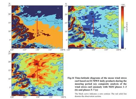
In summary, the 40-day variation in NEC/NEUC volume transport was closely related to the MJO.Specif ically, in MJO phases 1-3, the local wind f ield generated a negative wind stress curl anomaly near the 130°E section, which weakened the tropical gyre and the Mindanao Dome and, f inally, resulted in a weaker NEC and stronger NEUC. However, the cases were opposite in phases 5-7. The tropical gyre was enhanced when a positive wind stress curl anomaly occurred, corresponding to an increase in the NEC and a decrease in the NEUC.

5 SUMMARY AND CONCLUSION

Historically, few directly ADCP observed velocity data have been used to estimate the volume transport.The NEUC volume transport is particularly understudied. Recently, scholars have used mooring observation data to analyze the velocity structure of the NEC and NEUC. However, the focus has primarily been on the variation in velocity (Wang et al., 2015,2019; Zhang et al., 2017) rather than volume transport.This work focuses on the latter and studies its variability.

In this study, the mean structure and intraseasonal variability of the NEC/NEUC volume transport were investigated over the course of 365 days, with specif ic ADCP measurements taken at 8.5°N, 11°N, 12.5°N,15°N, and 17.5°N along 130°E. In addition, we also utilized other datasets to enhance the analysis,including satellite altimetry product data, RG-Argo data, WOA data, ECMWF wind daily data, and the MJO index. The main f indings can be summarized as follows:

The mean NEC and NEUC volume transports calculated from the mean velocity structures in the upper 950 m are 39 and 6 Sv, respectively. Analyzing the daily data, the volume transport of the NEC was estimated to be 52 (±14) Sv, with a maximum volume of 83 Sv. The volume transport of the NEUC corresponds to 18 (±13) Sv, with a maximum volume of 61 Sv.

Both NEC and NEUC volume transports have a signif icant 40-day variability. Overall, the ISV of the NEC is vertically coherent with that of the NEUC,which indicates that it is a primarily barotropic signal.

The NEUC was determined to have three cores,with centers located at 8.5°N (～500 m), 12.5°N(～700 m), and 17.5°N (～900 m), of which the middle core (12.5°N) was the strongest. The depth of the three cores gradually increased as the latitude increased.

Composite analysis suggested that the 40-day variability of the NEC and NEUC is related to the variability of the local wind stress curl anomaly between the various MJO phases. When the local wind f ield generates a negative (positive) wind stress curl anomaly, it results in a weaker NEC (NEUC) and a stronger NEUC (NEC).However, issues remain to be addressed. The spatial resolution of the mooring observation data was insuffi cient. Specif ically, the average latitudinal gap was 2.25°N between each mooring site, which was inadequate for structural reconstruction of the NEUC. Therefore, the exact latitude of each core needs to be further explored. Additionally, as mentioned above, the volume transport of the NEC and NEUC may have seasonal variability, which cannot be suffi ciently studied with current data across a one-year period. These issues need to be further studied in the future.

6 DATA AVAILABILITY STATEMENT

The datasets generated and/or analyzed during the current study are available from the corresponding author on reasonable request.

7 ACKNOWLEDGMENT

We would like to thank anonymous reviewers for their helpful comments and suggestions that improved the manuscript.