Simulating the Effect of Temperature Gradient on Grain Growth of 6061-T6 Aluminum Alloy via Monte Carlo Potts Algorithm
2021-11-05QiWuJiananLiLianchunLongandLinaoLiu
Qi Wu,Jianan Li,Lianchun Long and Linao Liu
Faculty of Materials and Manufacturing,Beijing University of Technology,Beijing,100124,China
ABSTRACT During heat treatment or mechanical processing,most polycrystalline materials experience grain growth,which significantly affects their mechanical properties.Microstructure simulation on a mesoscopic scale is an important way of studying grain growth.A key research focus of this type of method has long been how to efficiently and accurately simulate the grain growth caused by a non-uniform temperature field with temperature gradients.In this work,we propose an improved 3D Monte Carlo Potts(MCP)method to quantitatively study the relationship between non-uniform temperature fields and final grain morphologies.Properties of the aluminum alloy AA6061-T6 are used to establish a trial calculation model and to verify the algorithms with existing experimental results in literature.The detailed grain growth process of the 6061-T6 aluminum alloy under different temperature fields is then obtained,and grain morphologies at various positions are analyzed.Results indicate that while absolute temperature and duration time are the primary factors determining the final grain size,the temperature gradient also has strong influence on the grain morphologies.The relationships between temperatures,temperature gradients and grain growth process have been established.The proposed MCP algorithm can be applied to different types of materials when the proper parameters are used.
KEYWORDS Grain growth;temperature gradient;polycrystalline materials;Monte Carlo method;aluminum alloy
1 Introduction
Grain growth—the increase in the size of grains(crystallites)in a material at high temperature is the most common microstructural evolution process in polycrystalline materials such as pure metals,alloys and some ceramics.Grain size has an important influence on the mechanical,physical and chemical properties of polycrystalline materials,and is one of the most important microstructure parameters.During the preparation,forming,processing and welding of polycrystalline materials,long-time high temperature and deformation treatments are typically introduced.Under high temperature and deformation conditions,polycrystalline materials will experience the grain growth phenomenon.Therefore,the study of the grain growth process under thermal conditions is an important research field.Compared with experimental observations,simulation has advantages such as low cost,flexibility and the ability to performin situanalysis[1–3].
Monte Carlo Potts(MCP)and cellular automata(CA)methods are two algorithms commonly used by researchers for the simulation of evolving microstructure systems in mesoscopic scales.The MCP and CA methods originated from statistical physical simulation and computer simulation of self-reproducing systems[4–6],respectively,and they have been applied in the field of computational materials science since the 1980s[5,7,8].Since the initial simulation of uniform grain boundary motion and grain coarsening in the 2D and 3D spaces,many researchers have applied MCP and CA methods to more complex microstructure evolutions to continually improve the accuracy and applicability of the models.The MCP and CA models were used to simulate the nucleation and growth of recrystallized grains in the early stages[7,9],and the predictions were usually consistent with the experimental results.On the basis of uniform grain growth,some scholars developed the anisotropic grain growth and abnormal grain growth simulations by changing the surface energy distribution or energy calculation method of the Hamilton equations in the MCP and CA formulas[10,11].With the increasing complexity of simulation conditions,Gao et al.[12]established an actual time-temperature relationship model.Zinovieva et al.[13]studied the mesh anisotropy problem in CA models.Vertyagina et al.[14]improved the CA method so that it can be applied to materials with different space lattice forms.Rodgers et al.[15]used a rejection kinetic Monte Carlo model to simulate grain evolution in the welding process.In their work,a temperature-dependent grain boundary mobility termM(T)was introduced in an attempt to solve the difficulties of temperature inhomogeneity.Yang et al.[16]considered the selection probabilities for lattice site as a temperature-related value,and by this method,the grain orientations at higher temperature locations are updated more frequently.Other numerical calculation methods have also been combined to improve the analysis ability for temperature or deformation fields,such as FE-CA algorithms[17]and CA-lattice Boltzmann models[18].In recent years,as the CA and MCP methods were further developed,they have been applied in fields such as grain evolution simulation in welding pools[19,20],and solid-state friction stir welding joints[21,22],laser treatment and additive manufacturing[18,23].The efficient simulation of grain growth in heterogeneous and complex temperature fields is still a problem that limits the predictions of evolving microstructure systems.Microstructure evolution regulations and grain morphology need more detailed and quantitative studies,particularly in the 3D condition,which is closer to the actual evolution process.
By combining the MCP determination algorithm with CA formulations,this work proposes a 3D Mote Carlo Potts model to simulate the microstructure evolutions of AA6061.The model deals with inhomogeneous temperature fields by defining different iterating numbers at lattice sites with different temperature values.The influence of temperature gradients on grain boundary migration,grain size evolution and grain morphology is studied in detail.This work provides reference for further applications of simulation in various complex manufacturing processes involving temperature gradients.
2 Description of Model
The model uses 3D equilateral cube grids to mesh the spatial region.The shape of the simulated area is a cuboid or a cube,and the mesh model can be marked as m × n × p according to the grid numbers of each direction in the rectangular coordinate system.The actual spatial length corresponding to each lattice cell is marked asλ,which indicates the accuracy in the dimensions of the model.In the MCP model,each lattice cell is given an integer numberqto represent the value of grain orientation degree;these integers are limited from 1 to a positive numberNq.The model adopts Moore’s neighbor scheme;that is,there are 26 adjacent neighbor cells around each central cell.When the grain orientation degrees of adjacent cells are the same,the model considers that these cells constitute the same grain.If the grain orientation degrees of adjacent cells are different,the grain boundaries are formed.According to this rule,the average intercept method is used to estimate the average spatial grain sizel,

whereLis the length of a line,andNgis the number of grains found along this line.Lines used to calculatelare all drawn parallel to the coordinate axis.
The essential driving forces during grain growth of polycrystalline materials are atomic motion and grain boundary migration under high temperatures[24].When the energy caused by temperature rise for the material exceeds the energy threshold to overcome energy barriers,atomic migration and atomic transition will occur,which finally results in grain boundary movement and grain growth.The simulation of grain growth is achieved by simulating the ordered transformations of grain orientation degrees in this MCP model.Transformation criteria combined with curvature-driven mechanisms and energy rules are used to determine the ordered change of grain orientation degrees at every lattice cell.
The curvature-driven transition criterion is proposed based on the grain growth law summarized from theoretical analysis,numerical simulation and experimental observations[25].On 2D sections,the grain growth of adjacent grain boundaries tends to be a stable shape with an angle of 120 degrees,particularly when the grain boundary energy is homogeneous,i.e.,regular hexagonal shapes[26].This trend can be described by the curvature driven mechanism.In the 3D model,26 Moore-type neighbor cells around each central cell are divided into four groups to judge the curvature-driven transition criteria.As shown in Fig.1a,the group 1 is composed of nine adjacent cells at the same plane,and it can be seen that there are six equivalent planes adjacent to the central cell.Group 2 is composed of six cells that are coplanar with the central cell,as shown in Fig.1b.In the same way,according to the distance relationship,another group of 12 and 8 cells sharing edges and vertices with the central cell form Group 3 and Group 4,respectively,as shown in Figs.1c and 1d.The judgment priority is from Group 1 to Group 4 in turn,and when the MCP model is running according to the curvature-driven transition criterion,it is judged according to the following four conditions in sequence:
(a)If there are two or more lattice cells with an equivalent degree of grain orientation in Group 1,then the central cell will be changed to the same value.
(b)If there are four or more lattice cells with an equivalent degree of grain orientation in Group 2,then the central cell will be changed to the same value.
(c)If there are eight or more lattice cells with an equivalent degree of grain orientation in Group 3,then the central cell will be changed to the same value.
(d)If there are five or more lattice cells with an equivalent degree of grain orientation in Group 4,then the central cell will be changed to the same value.

Figure 1:Groups of adjacent cells,(a)Group 1,(b)Group 2,(c)Group 3,(d)Group 4
When the above criteria(a)to(d)are judged in sequence,as long as one condition is satisfied,the subsequent judgments will not be continued.If all the conditions are not met,the curvaturedriven transformation rule will be foregone and at the same time the energy rule will continue.The energy rule is based on the principle that,during grain growth,total grain boundary energy and total grain boundary areas always tend to be decreased.For each lattice cell i,its free energyEiis calculated by Hamilton formula[16],
Now this strange friendship was observed by the Tanuki, a wicked, quarrelsome beast, who hated the peasant, and was never tired of doing him an ill turn

whenJiis a function representing unit grain boundary energy of lattice cell i,and j represents one of the neighbor lattice cells around i.δis the Kronecker function,and if grain orientation degreeqiis equal toqj,then the value ofδijequals 1;ifqiis not equal toqj,then its value will be 0.Using Eq.(2),the total energy of the systemE1can be calculated from the summation of all cells.For a certain central lattice cell,if the grain orientation degree is transformed to a randomly selected neighbor cell,then the new total energy is denoted byE2.The change of total energy can be then calculated by

Then,a probabilitypbased on the variation of total energy is used to determine whether to accept the above transformation,

wherekBis Boltzmann constant andTabsis absolute temperature.In this model,the value of termJi/kBTabsis assumed to be 1 during the numerical calculations[21],and it is proved that this assumption does not affect the simulation results of real physical processes[4,6].It is worth noting that the curvature criterion will lack the necessary neighbor cells to form four groups at the boundaries of the grids systems,and the energy rule will also lack sufficient calculation cells at the boundaries of the simulation region.In this work,the remedy for this issue is to use periodic boundary conditions.At the boundaries of the simulated region,the model is set as a cyclically symmetric boundary condition.That is,to assume the upper surface is in contact with the lower surface,the left surface is in contact with the right surface,and the front surface is in contact with the rear surface.
Fig.2 shows the above calculation process for every central cell.In this work,one such re-orientation iteration is a basic computing unit of the MCP algorithm.The number of reorientation times for the cell located atijkis marked asReijk.The total re-orientation attemptsRetolfor the grid system can now be obtained by

During the simulation process,a cell with location ijk will be chosen randomly and perform the re-orientation iteration once.The program will cycle to select cells at random locations until all cells are selected to run the specific re-orientation timesReijk.

Figure 2:Flowchart of re-orientation criterion
To simulate an actual grain growth procedure,particularly the non-uniform grain growth with temperature gradients,it is necessary to establish the relationship between time,temperature and re-orientation times for each specific cell.This means material grains represented by discrete cells related to different temperature curves should be modeled by differentReijkduring the simulation of microstructure evolution.

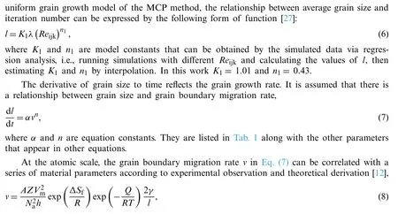
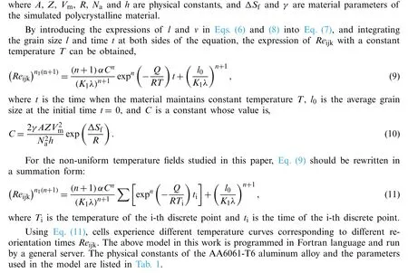
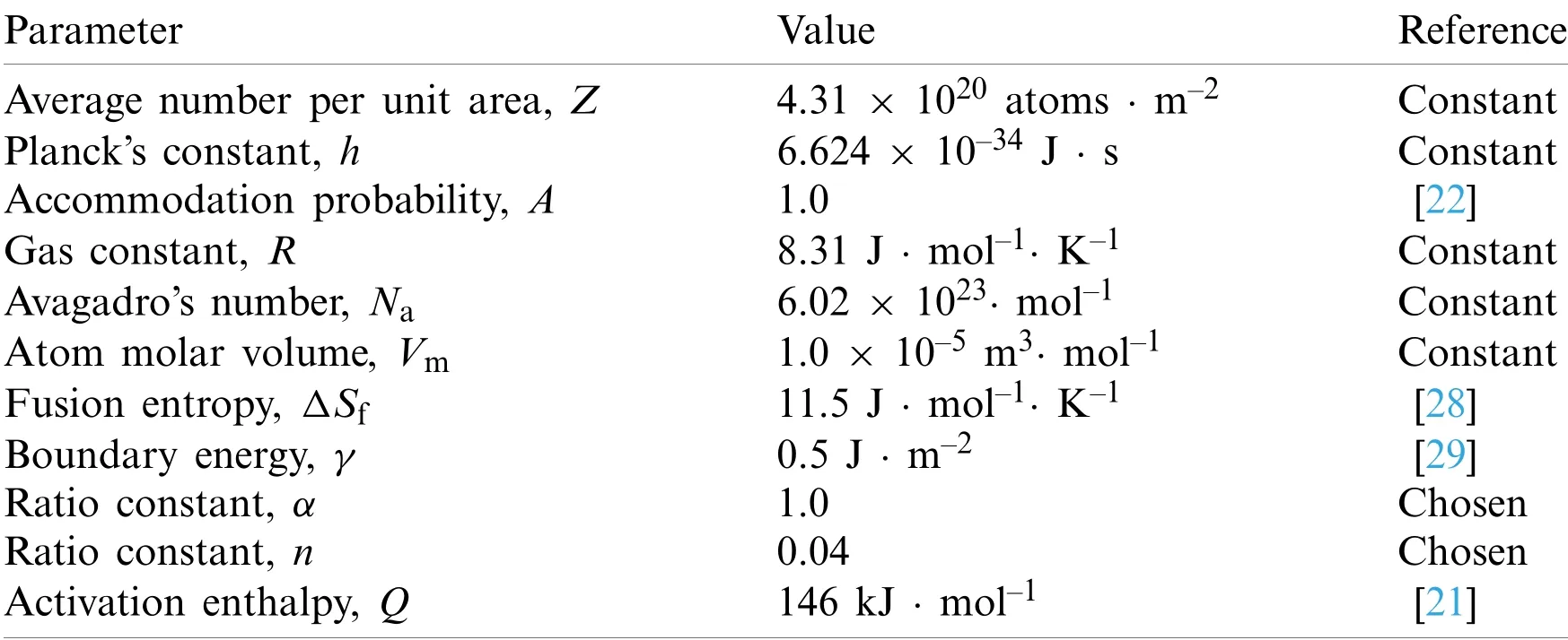
Table 1:Material parameters and model constants
3 Results and Discussion
3.1 Analysis of Grid Dimension and Resolution
Grid dimension is an important parameter for the MCP model,because it determines the calculation efficiency,cost and simulation region.To study the sensitivity of the model to the number of cells,five cases with different scales and proportions of total grids were selected to simulate the grain growth with fixed iteration steps.The scales of the five models were 200 × 200× 200,300 × 300 × 300,350 × 350 × 350,400 × 400 × 400 and 500 × 500 × 300,respectively.The total number of cells were 8,27,42,64 and 75 million,respectively.During our study of the sensitivity of grid dimension,the material properties and temperature were not considered.Reijkwas fixed at a relatively large number of 10000 for all cases,which meant that grain growth process was uniform.Initially,the grain orientation degrees in each model were assigned randomly,andNqvalues were set at 100.The length of each lattice cellλwas defined as 1 μm during the simulation.
The simulation results showed that the predicted final grain sizes in the five cases were very close.The average value of grain sizes obtained was 50.89 μm,and the overall standard deviation was only 0.95 μm.Fig.3 shows the grain growth curves;the horizontal ordinates are obtained from the average re-orientation times of all cells during the simulation.It can be seen that the trends of grain growth are highly consistent.At the initial stage,the average grain size was small,so the total area and energy of grain boundaries are were high,which led to a high rate of grain growth.With the increase of re-orientation iterations,the grain growth rate decreased and grain size tended to converge.The logarithmic values ofReijkand average grain sizelwere calculated for each of the five cases,respectively,and the ratio log10(l)/log10(Reijk)was called the grain growth exponent.The theoretical value of normal grain growth exponent was 0.5[30].In these five cases,the average grain growth exponent was 0.44,which was close to the theoretical value.When the fifth case with a scale of 500 × 500 × 300 was compared to the other four cases,it indicated that reducing the number of grids in one of the three dimensions did not affect the grain growth simulation process.Therefore,for a specific case,the cost of computation could be reduced significantly by reducing the number of grids along one specific direction without influencing the simulation process.

Figure 3:Grain growth curves with different model dimensions
Cell space lengthλdefines the resolution of the model,and influences the calculation ofReijkfor every cell according to Eq.(11).The model with grid system 200 × 200 × 200 described above was used to investigate the influence ofλ,and three values—0.5,1 and 2 μm—forλwere compared.Exponential growth curves with different values ofλare illustrated in Fig.4.It can be seen that changing the value ofλdoes not affect the overall trend of grain growth,but affects the grain growth rate calculated in the model.To grow to the same grain size,the model with smallλneeds more re-orientation iteration times.Because the model parameterλhas been considered in the formula for calculatingReijk,whenλis reduced,the calculatedReijkvalue will increase proportionally,so that it can make up for the difference caused by different resolutions.In other words,when the higher resolution model with smallerλis used,the re-orientation times will be increased correspondingly to ensure the accuracy of the model.

Figure 4:Exponential growth curves with different values of λ
3.2 Validation of Model
To verify the accuracy of the model and debug the parameter settings,the proposed algorithm was used to establish prediction models of grain growth for materials experiencing different thermal histories.Then the predicted values were compared with experimental and numerical results in the literature.The observed results of grain growth in friction stir spot welding(FSPW)of 6061-T6 aluminum alloy by Gerlich et al.[31]were selected as verification.During the FSPW process,the grains in the welding seam were crushed and refined by mechanical stirring,and then the grains recrystallized completely to form fine and compact equiaxed grains.Driven by the heat generated from spot welding,the grains in the welding seam continued to grow after the mechanical stirring.According to the grain evolution characteristics of FSPW,a 200 × 200× 200 cube model was used to simulate the grain growth process in a welding seam.The actual space length of the lattice system was chosen asλ= 0.2 μm,because the grain sizes are usually very small.Grain orientation degree values were initially randomly assigned in the model.Four temperature curves were simulated and compared,as shown in Fig.5,which corresponds to the temperature curves of quenching treatment under four different welding conditions.Fig.5 also shows two electron backscatter diffraction(EBSD)grain maps that can be compared with the predicted grain images.TheReijkcorresponding to the four temperature curves calculated by this algorithm were 78,131,212 and 266,respectively.Fig.6 shows the distribution of final grain size and morphology simulated by the MCP model,where grain morphology is displayed via randomly assigned corresponding color values to all grain orientation degrees from 1 toNq.It can be seen from the grain morphology that the grains are equiaxed and that grain size increases with the increase of temperature.The predicted results are in agreement with those of experimental observation and empirical calculation.The maximum error is only 6.79%,which verifies that the algorithm and parameters in this paper can predict the grain growth process of AA6061-T6 with heat treatment.Before the formal simulation experiment,through the above comparison with the experimental results in the literature,the parameter settings of the model were further debugged to ensure that the simulation results are consistent with the actual situation.

Figure 5:Different thermal history curves used for validations[31]
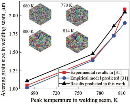
Figure 6:Comparison of predicted results with literature
3.3 Influence of Temperature Gradients
The most direct impact of an inhomogeneous temperature field on grain growth is the presence of temperature gradients.Temperature gradients cause the differences in atomic migration rates and grain boundary energies between adjacent grains in the studied region,which affects grain growth.The MCP method in this work is used to quantitatively analyze the effect of temperature gradients on grain growth.
The actual modeled physical condition in this work is grain coarsening of polycrystalline materials driven by temperature field from an equiaxed fine grain state.In practice,the initial fine grain state can be obtained from solidification,recrystallization or a mechanical machining process.However,this model only simulates the nonuniform grain coarsening process under subsequent heat treatment conditions.In the MCP model,the initial grain distribution is generated by randomly assigning grain orientation degree values to all lattice cells.The rectangular coordinate system is composed of three directions by the simulated cuboid region,which are marked as the I,J and K directions.The non-uniform temperature field is set to change only along the I direction,which means that the vector of the temperature gradient is along the I coordinate.To reduce the overall calculation cost and improve the computational efficiency,the number of grids at the J direction has been reduced appropriately.In the study,the size of the MCP model is 400 ×50 × 400 with a total of 8 million lattice cells,and the cell space length of each single cell is defined as 1 μm.Four temperature distribution conditions are designed.At the locations of I= 1,the temperatures for all four cases are set at 300 K,which is relatively low and obviously unable to stimulate grain growth.At the far side of the grid where I = 400,the temperatures are set at 430,560,690 and 823 K for the four cases,respectively.These values are selected in proportion from room temperature(300 K,I = 1)to the temperature near the melting point of AA6061-T6.Temperature fields are designed as linear distribution along the I direction at the rest of the locations in the simulation region.The duration of the four thermal conditions is assumed to be 100 seconds.Taking the number of grids as the length unit,the simulated four temperature gradients vary from 0.343 K/grid to 1.308 K/grid,as shown in Fig.7.

Figure 7:Different temperature gradients simulated
According to the method proposed in this work,the number of re-orientation iterations for all cells in the simulation area can be calculated before running the MCP model.Fig.8 illustrates the number of re-orientation iterations at different locations along the I direction under different temperature gradient conditions.At position I = 1,the temperatures of cells are only 300 K,and therefore theReijkvalues are low,at 62.With the change of positions along the I direction,the temperatures of each condition increase linearly,and the calculatedReijkvalues also show an increasing trend.TheReijknumber reaches the highest values at the right boundary where I = 400.In Condition 1 of temperature gradient,the maximum number of iterations at the end is only 300 because the highest temperature is only 430 K.In Condition 4 of temperature gradient,the maximum temperature at the right boundary is close to the melting point of 6-series aluminum alloy,reaching 823 K,and the corresponding number of iterations is 1917.At the same time,it can be seen from the diagram that theReijkvalues do not increase linearly with position I under all four thermal conditions.In Case 4,which has higher temperature and temperature gradient values,the increasing rate ofReijkis also faster,which shows an obvious non-linear characteristic.

Figure 8:Re-orientation times at different locations along I direction
Fig.9 shows the distribution of grain morphology at the final time 100 s for the four temperature gradient conditions.The left end corresponds to I = 1 and the right end corresponds to I = 400.It can be seen that the 3D MCP model performs well at simulating the spatial growth of AA6061-T6 grains.The grain morphology shows grains with nearly the same grain size at the same I coordinate positions,and there is a significant gradient distribution of grain size along the direction of I.At the position I = 1,the grain sizes are relatively small,and at the position I =400,the grain sizes reach the largest values.In condition 1,the grain size changes slowly along direction I,while in condition 4,because of the large temperature gradient along the I direction,the temperature changes quickly with the position and the grain coarsens rapidly.It can also be seen in Fig.9 that although the temperatures at the leftmost end are all 300 K in four thermal conditions,the grain sizes vary slightly at I = 1 due to the different temperature values in the adjacent areas.This predicted phenomenon indicates that grain growth is regional and there exist interactions between adjacent areas with different temperature distributions.

Figure 9:Visualizations of predicted final grain structures,(a)Gradient 1:0.343 K/grid,(b)Gradient 2:0.685 K/grid,(c)Gradient 3:1.028 K/grid,(d)Gradient 4:1.308 K/grid
To further analyze the grain growth in the simulated area,2D cross-sections are used to observe the grain morphology.Through the central cell of each model region,cross-sections perpendicular to the three coordinate axes are built,and grain boundaries are represented by blue lines.The 2D grain morphology of different thermal conditions at different directions is then obtained,as shown in Fig.10.The grain morphology on the 2D cross-sections conform to the 3D actual grain morphology,presenting an approximate equiaxed hexagon shape.Most of the grains are formed with 120◦angles at the grain boundaries,which are consistent with many experimental observation results[5,32,33].The distribution of grain size is relatively uniform.There are a few fine grains that have not been coarsened or merged around the larger grains.On the IK plane perpendicular to the J-axis and on the IJ plane perpendicular to the K-axis,the grains are gradient-distributed along the I direction.On the KJ plane perpendicular to the I coordinate axis,it can be seen that the grain size distribution is almost uniform,indicating that at the positions with the same I coordinates,grain size distribution is not affected by the temperature gradient.For thermal condition 1,the grain size is smaller due to the lower overall temperature.As the temperature gradient increases,e.g.,in Conditions 2–4,the grain coarsening rate along the I direction increases significantly,and much larger grain sizes are obtained.
The average intercept method described in Eq.(1)can be used to estimate the grain size on any straight line or plane.Fig.11 shows the distribution of grain size along the I direction for the simulated four cases.At the left end where I = 1,the grain size values are low for all four thermal conditions.As the I position changes,the temperature increases and the grain coarsens rapidly.In Condition 4 with the large temperature gradient,the grain coarsening rate along the I direction is the highest.At the position of I = 400,the grain sizes reach 8.63,14.03,19.08 and 27.61 μm,respectively,in the four cases.The results show that the smoothness of the four curves are significantly different.The grain size curve of Condition 1 is relatively gentle,while the fluctuation in grain size increases with the increase of the temperature gradient.On the grain size curves of thermal Conditions 2–4,some obvious grain size decreasing sections can be observed.This is because when the temperature and temperature gradient are higher,the grain boundary migration rate is higher,and the grain growth is more complex and random,resulting in the existence of small grains that are not coarsened or merged at some of the local parts.Because large grains and some small grains exist at the same time,the fluctuation in size occurs in the high temperature region when the intercept method is used to calculate the grain size.It is also found that the spatial gradient of grain size increases with the increase in the spatial gradient of temperatures.
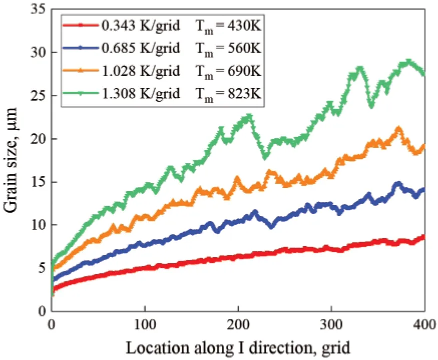
Figure 11:Curves of grain sizes along I coordinate
The distribution of grain size under the four temperature gradient conditions is shown in Fig.12.It can be seen that,when influenced by the linear temperature gradients,the distribution of grain size shows obvious single peak distribution characteristics in the four conditions,and the appearance frequency of grain size decreases rapidly with the increase in sizes.When the temperature gradient is 0.343 K/grid,the total number of grains reaches 4793,and the maximum grain size is 23.35 μm.When the temperature gradient rises to 1.308 K/grid,the total number of grains decreases to 684,and the maximum grain size increases to 60.59 μm.Comparing Fig.12a,12b with 12c,12d,it can be seen that as the numbers of peak values of grain size increase,the fluctuation as well as the grain size dispersion increase.This proves that with the increase in temperature gradient,the trends of abnormal grain growth and abnormal size distribution increase.

Figure 12:Grain size distribution in four cases.(a)Gradient 1,Tm= 430 K,(b)Gradient 2,Tm=560 K,(c)Gradient 3,Tm= 690 K,(d)Gradient 4,Tm= 823 K
The variation in the grain boundary area from numerical simulation is shown in Fig.13.The grain boundary area is the same under all conditions at the initial time.During the grain growth driven by temperature field,the grain boundary area gradually decreases,and the rate of reduction in all conditions slows down,which is consistent with the law of grain growth rate slowing down in Fig.3.It can also be seen that under high temperature gradient conditions,the rate of reduction is much higher than that under low temperature gradient conditions,which is consistent with the phenomenon shown in Fig.12,that the fraction of small grains is lower under high temperature gradient conditions.This is due to the high level of system energy.

Figure 13:Evolution of grain boundary areas with different temperature gradients
4 Conclusions
The proposed 3D Monte Carlo Potts(MCP)method can simulate the grain growth driven by spatial non-uniform temperature field for the AA6061-T6 aluminum alloy.Based on the physical quantitative calculation formula of grain boundary transition rate,the proposed method correlates thermal histories with re-orientation iteration steps of the MCP model induced by non-uniform temperature fields.Grid scales of the MCP model were tested and proved to have little effect on the process of grain growth simulation.Different model resolutions can be balanced by reorientation iteration times in this algorithm.In the 3D model,reducing the grid dimension along a certain direction does not significantly affect the analysis results.In this work,the simulation results based on physical parameters of 6061-T6 aluminum alloy have been proved to have a relatively low error rate compared with experimental results in literature.When the physical parameters of different polycrystalline materials are selected,the proposed method is applicable to other materials as well.
The two main factors affecting the final grain size under heat treatment are the absolute temperature and the corresponding time duration.Temperature gradient is the main factor affecting the grain growth uniformity and morphology distribution of polycrystalline materials.When the temperature gradient distribution caused by heat treatment is low,the final results of coarsened grain distribution tend to be equiaxed and flat.When the polycrystalline material is processed with the condition of large temperature gradient,the transition from fine grain area to coarse grain area is very rapid.At the same time,under high temperature and high temperature gradient conditions,the simulation results will be more local irregular grain distribution,and even local abnormal grain coarsening that the estimated average grain size decreasing with the increase of temperature.
Funding Statement:The authors would like to acknowledge the financial support from China Postdoctoral Science Foundation Project(2018M641128)and the National Key Research and Development Program of China(2018YFB0703500).
Conflicts of Interest:The authors declare that they have no conflicts of interest to report regarding the present study.
杂志排行
Computer Modeling In Engineering&Sciences的其它文章
- Determinantal Expressions and Recursive Relations for the Bessel Zeta Function and for a Sequence Originating from a Series Expansion of the Power of Modified Bessel Function of the First Kind
- Study of Degenerate Poly-Bernoulli Polynomials by λ-Umbral Calculus
- The New Neutrosophic Double and Triple Exponentially Weighted Moving Average Control Charts
- Neutrosophic N-Structures Applied to Sheffer Stroke BL-Algebras
- Weighted Parameterized Correlation Coefficients of Indeterminacy Fuzzy Multisets and Their Multicriteria Group Decision Making Method with Different Decision Risks
- Subdivision Surface-Based Isogeometric Boundary Element Method for Steady Heat Conduction Problems with Variable Coefficient
