Modelling on seasonal lake ice evolution in central Asian arid climate zone: a case study

LU Peng, Bin CHENG, Matti LEPPÄRANTA & LI Zhijun

1 State Key Laboratory of Coastal and Offshore Engineering, Dalian University of Technology, Dalian 116081, China;

2 Finnish Meteorological Institute, Helsinki Fi-00101, Finland;

3 University of Helsinki, Helsinki Fi-00014, Finland

Abstract The seasonal cycle of ice thickness and temperature in Lake Wuliangsuhai, a typical shallow lake in the central Asian arid climate zone, was simulated using the HIGHTSI model and the MERRA-2 data as the meteorological forcing. The average ice growth rate was 0.64 cm·d-1 and -1.65 cm·d-1 for the growth and melting stage of the ice cover, respectively. The ice thickness agreed well with the field observations conducted in winter 2017, with a correlation coefficient of 0.97. The ice temperature field also agreed with observations in both daily variations and the vertical profile, and a better agreement in the daily amplitude and profile shape of ice temperature could be achieved if field data on physical properties of snow cover and melting ice were available. This study proved the feasibility of both the HIGHTSI model and the MERRA-2 data for modeling the ice cover evolution in Lake Wuliangsuhai, providing a basis for a deep insight into the difference of lake ice evolution between central Asian arid climate zone and polar/sub-polar regions.

Keywords lake ice, HIGHTSI model, ice thickness, ice temperature

1 Introduction

In the Northern Hemisphere, approximately half of the inland surface waters freeze over every year, and the duration of ice cover has a major role on local climate(Downing et al., 2006; Kirillin et al., 2012). Compared to other cold climate terrestrial surfaces, lakes have a higher evaporation rate (Rouse et al., 2008) and less day-and-night temperature variability. The ice season has impacts on both the regional climate and weather events, such as thermal moderation and the lake effect on snow accumulation(Prowse et al., 1990; Brown and Duguay, 2010). Previous studies have shown that ice seasons have generally become milder, resulting in a shorter duration and thinner ice cover(Magnuson et al., 2000; Leppäranta et al., 2017; Hewitt et al., 2018; Solarski and Rzętała, 2020).

Similarly with polar and sub-polar lakes, which have attracted many attentions (Kirillin et al., 2012; Cheng et al.,2014), lakes in the cold and arid climate of Central Asia are frozen for several months of the year. But Central Asia has many obvious differences from the northern areas in the growth and decay of the lake ice cover. There, for example,the incident solar radiation keeps at a high level throughout winter because of the high solar elevation angle at noon(30°-55°) and continuously sunny days in winter.Additionally, the snow cover on ice is always very thin or absent due to low winter precipitation. In recent years,research on ice-covered lakes has increased in Central Asia,and several new phenomena in the limnology of freezing lakes have been discovered. Shi et al. (2014) found that the thermal diffusivity increases slowly with decreasing ice temperature in a thermokarst lake. Huang et al. (2019)reported a high heat flux from water to ice in a lake located on the central Qinghai-Tibet Plateau. Su et al. (2019)reported the impact of global warming with later ice-on and earlier ice-off dates in Qinghai Lake. However,investigations on ice thickness and temperature in central Asian lakes are still very limited (Huang et al., 2019), and their differences from polar/sub-polar lakes is not yet clear.

Field observations are the first choice to address this issue, but the challenge comes from the difficulty with observing the complete process of lake ice growth and decay. Therefore, numerical simulations using lake ice models can be applied as powerful supplements to the limited field observations. Various lake models have been applied to perform numerical simulations of snow and ice(Vavrus et al., 1996; Wange et al., 2010; Yang et al., 2012;Cheng et al., 2014). Among them, the one-dimensional high-resolution thermodynamic snow and ice model(HIGHTSI) is well-calibrated and widely used (Semmler et al., 2012; Yang et al., 2012; Cheng et al., 2016). It is daily used in sea ice forecasting in the Finnish Meteorological Service, and it is also widely used in the simulations of seasonal formation and extinction of lake ice (Huang et al.,2019a) and other related studies. Compared with other lake ice models, the HIGHTSI model takes into account the coupling of the ice and snow layers, and also the internal melting within the ice layer (Cheng et al., 2014).

As the first step towards a deep insight into the difference of lake ice evolution between central Asian arid climate zone and polar/sub-polar regions, the motivation of this study was to investigate the evolution of thickness and temperature profile of the ice cover in Lake Wuliangsuhai in Inner Mongolia, for a typical shallow lake in central Asian arid climate zone. The HIGHTSI model was employed for this study and the modeling results were verified by limited in-situ observations.

2 Methodology

2.1 Site description

Lake Wuliangsuhai (40.9°N, 108.9°E) is located in the central part of Inner Mongolia, northern China. It is a representative shallow lake in the lake area of the Mongolian Plateau. Lake Wuliangsuhai covers an area of over 300 kmand its altitude is 1019 m above the sea level(Figure 1). The lake is 35.4 km long and 6.6 km wide, and the mean and maximum depths are 1.0-1.5 m and 2.5-3.0 m, respectively. The annual mean air temperature is 7.5 ℃ . The lake is frozen from early November to the end of March, and the average annual maximum ice thickness is 63 cm (Yang et al., 2016).

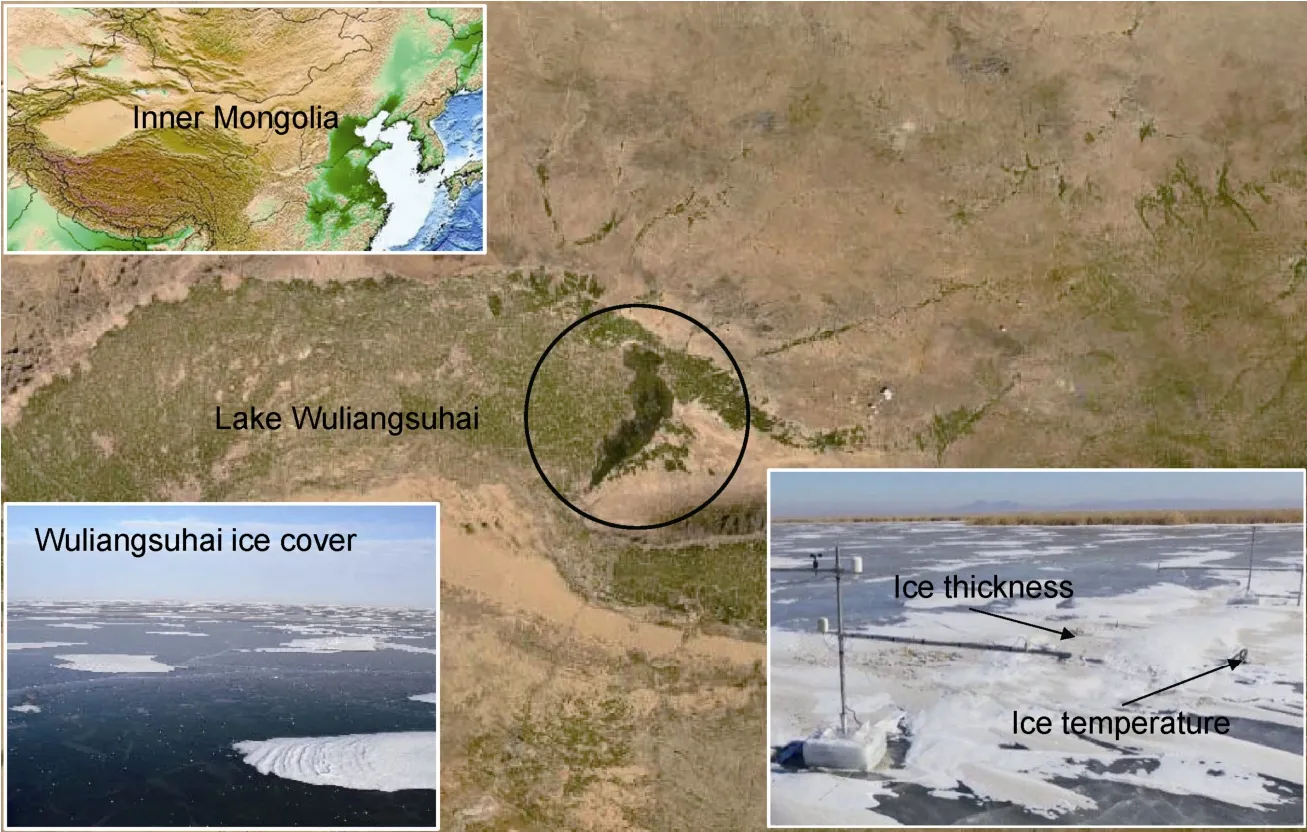
Figure 1 Location of Lake Wuliangsuhai. The lower left shows the ice cover on the lake, and the lower right shows the field site during winter 2017.

We conducted field observations in Lake Wuliangsuhai during winter 2017, including weather, ice thickness, and ice-water temperature profile (Figure 1). The detailed descriptions of the observations, equipment, and results were reported in Lu et al. (2020). The water depth was 1.7 m at the field site. Based on our previous field observation experience of Lake Wuliangsuhai, it was determined that the lake freezes around the beginning of December. The modeling start date was also determined to be 5 December based on the freezing degree day method.The variations of water level in winter are negligible,because no inflow or outflow is allowed then (Song et al.,2019).

2.2 Thermodynamic ice model

A well-calibrated and widely used thermodynamic snow and ice model HIGHTSI is applied in this study to investigate the lake ice thickness and temperature (Semmler et al., 2012; Yang et al., 2012; Cheng et al., 2016). The basic equations of the HIGHTSI model are shown below(Yang et al., 2012):

Eq. (1) controls the temperature conduction within the ice, and Eqs. (2) and (3) are the boundary conditions at the upper and lower surfaces. In Eq. (1),

T

is the ice temperature;

ρ

is the ice density;

c

is the specific heat of ice;

k

is the heat conduction coefficient of the ice, and

Q

is the solar radiation. In Eq. (2),

Q

, is the net long-wave radiation at the surface;

α

is the surface albedo; 1-

γ

is the fraction of surface absorption of solar radiation;

Q

is the sensible heat flux;

Q

is the latent heat flux;

Q

is the heat flux from precipitation;

F

is the heat conduction from the ice to the surface; and

F

is the equilibrium term of the surface heat flux. The heat flux pointing towards the surface of ice/snow is defined as positive, and calculations of each term in Eq. (2) can refers to Cheng (2002). In Eq. (3),

L

is the latent heat of freezing; ℎis ice thickness;

F

is the conductive heat flux from the water body;

T

is ice bottom temperature;

T

is the lake freezing temperature. In the HIGHTSI model,

F

is usually identified as a constant.Precipitation in the Lake Wuliangsuhai region is very low,and therefore the

Q

term in Eq. (2) can be neglected(Huang et al., 2019a).

2.3 Meteorological data and model parameters

The meteorological forcing data were obtained from MERRA-2 (The Modern Era Retrospective-analysis for Research and Applications) provided by NASA (National Aeronautics and Space Administration). It is a reanalysis dataset that includes long time-series of meteorological quantities, such as air temperature, wind speed, humidity,and radiation. MERRA-2 covers the whole world with a spatial resolution of 0.5° × 0.625° and a temporal resolution of 1 h. Therefore, it can be used directly in HIGHTSI model calculations.

Figure 2 shows the comparison between MERRA-2 and the field observations for the winter 2017, including air temperature, wind speed, and humidity. It can be seen that the air temperature of MERRA-2 is close to the measurements,with the mean bias of 0.94℃ and a correlation coefficient of 0.91. The mean bias between the wind speed of MERRA-2 and the measurements is 0.11 m·s, with a correlation coefficient of 0.62, and for the humidity these values are -16.26% and 0.69%. These accuracies are considered sufficient to use MERRA-2 data in the modelling the ice season in Lake Wuliangsuhai (Huang et al., 2019a).

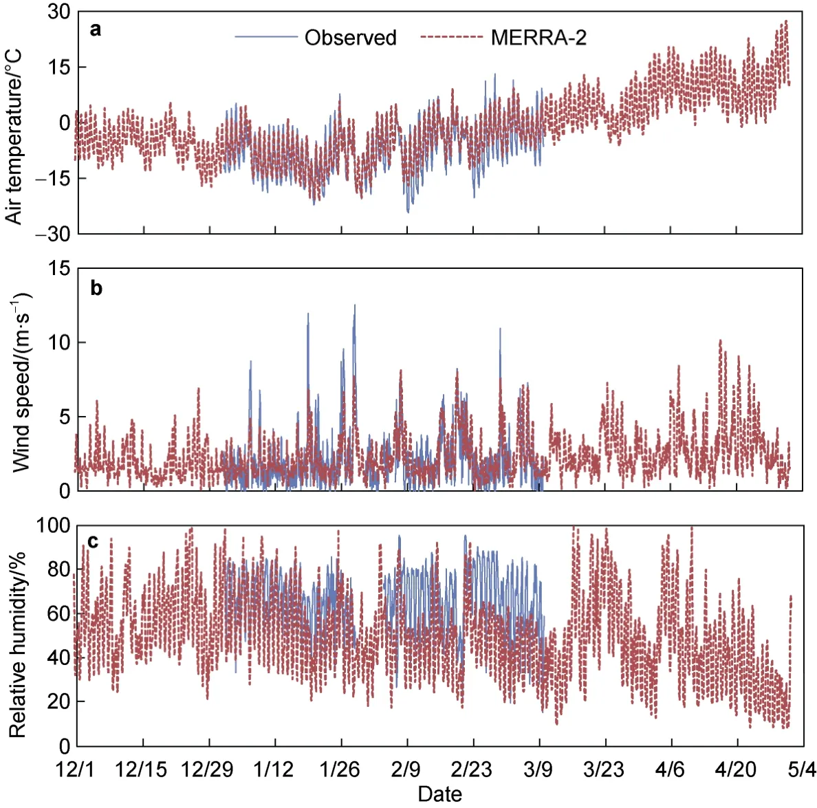
Figure 2 Air temperature (a), wind speed (b) and relative humidity (c) produced by MERRA-2 and comparisons with field observations.

Clouds were not considered during the modeling period because the sky was mostly clear over Lake Wuliangsuhai in winter. Moreover, the heat flux at the bottom of the ice was estimated from the field measurements (Lu et al., 2020). The standard thermal properties of ice was determined according to the average ice temperature that was -3.4℃ during observation period on Lake Wuliangsuhai in winter 2017 (Lu et al., 2010).Since the lake ice density was 2.5% less than the density of pure ice, the thermal properties of ice were modified according to ice density and air content (Leppäranta, 2014),as shown in Table 1.

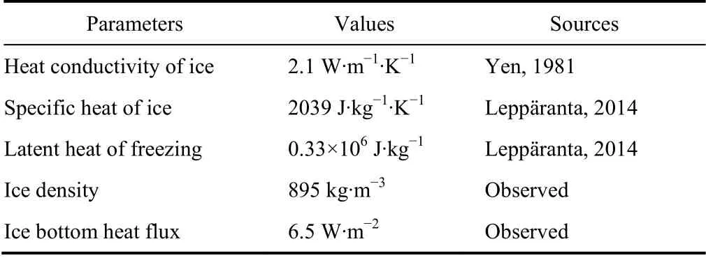
Table 1 The thermal properties of ice

3 Results and discussions

3.1 Lake ice thickness

The HIGHTSI model results on the cycle of ice thickness and temperature in a complete winter season are shown in Figure 3. Within the observation period from 1 January to 9 March, the correlation coefficient between modeling and observations is 0.97, and the average error is 0.01 m. It proves the feasibility and accuracy of the modeling using both MERRA-2 data and the HIGHTSI model.

In winter 2017, the ice thickness increased rapidly from 0 to 48 cm from 5 December to 24 January. From 25 January to 3 March, the ice thickness increased slowly from 48 cm to 56 cm. The average ice growth rate was 0.64 cm·d. After March 3, the ice began to melt at a rate of 1.65 cm·d, and the lake ice disappeared on 6 April.Because of the human intervention of opening the gates and releasing water during the melting period in spring, the end of ice period is always earlier than the date obtained from the pure thermodynamic model.

3.2 Lake ice temperature

A comparison between the modelled and measured ice temperature is shown in Figure 4. According to the deployment of the temperature probe, the temperature at the depths of 10 cm and 20 cm below the ice surface were selected, and the basic statistics of the comparisons are listed in Table 2. Similar to the ice thickness, the modelled ice temperature was close to the measured value, with the mean bias of 0.63℃ at the 10 cm depth and 0.09℃ at the 20 cm depth. The measured and modelled average ice temperature at 10 cm were -4.46℃ and -3.67℃, respectively, and at 20 cm the corresponding values were -3.68℃ and -2.62℃.The correlation coefficients were greater than 0.85 and the average error were less than 0.55℃, which further illustrates the high accuracy of the modelled results.

Table 2 The mean bias (MB), root mean square error (RMSE),correlation coefficient, and relative error between the modelled and observed ice temperature

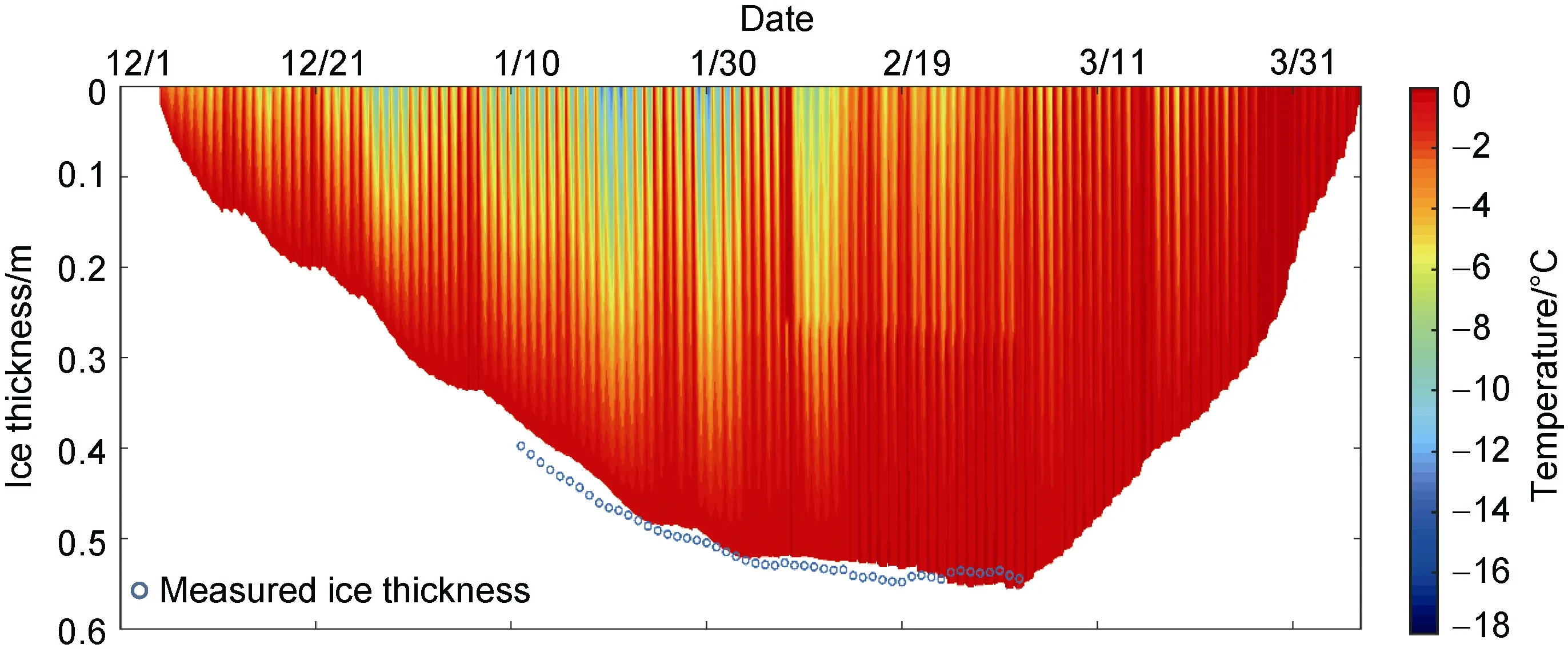
Figure 3 HIGHTSI modelled ice thickness, temperature (color scale) and measured ice thickness (circles) for winter 2017 in Lake Wuliangsuhai.

In Figure 4, the amplitude of the modelled daily ice temperature is close to the measured data in the early period,but in the later stage the modelled amplitude is much less than the observations. The modelled daily ice temperature difference at the 10 cm depth is close to the measured value before the snowfall on 8 February, with a deviation of 0.35℃ , while thereafter the deviation is -1.91℃ . The main reason is that in the model calculation the effect of snow on the ice temperature change needs to be revised. Due to the insufficient snow observations, with only snow depth measured, it is impossible to give proper physical properties of the snow cover, such as snow density, thermal conductivity and so on. These physical properties have an impact on the accuracy of the model results. The temperature at the 20 cm depth is less affected by snow, and the daily temperature difference of ice temperature before and after the snowfall is relatively close, with a deviation of 0.09℃.

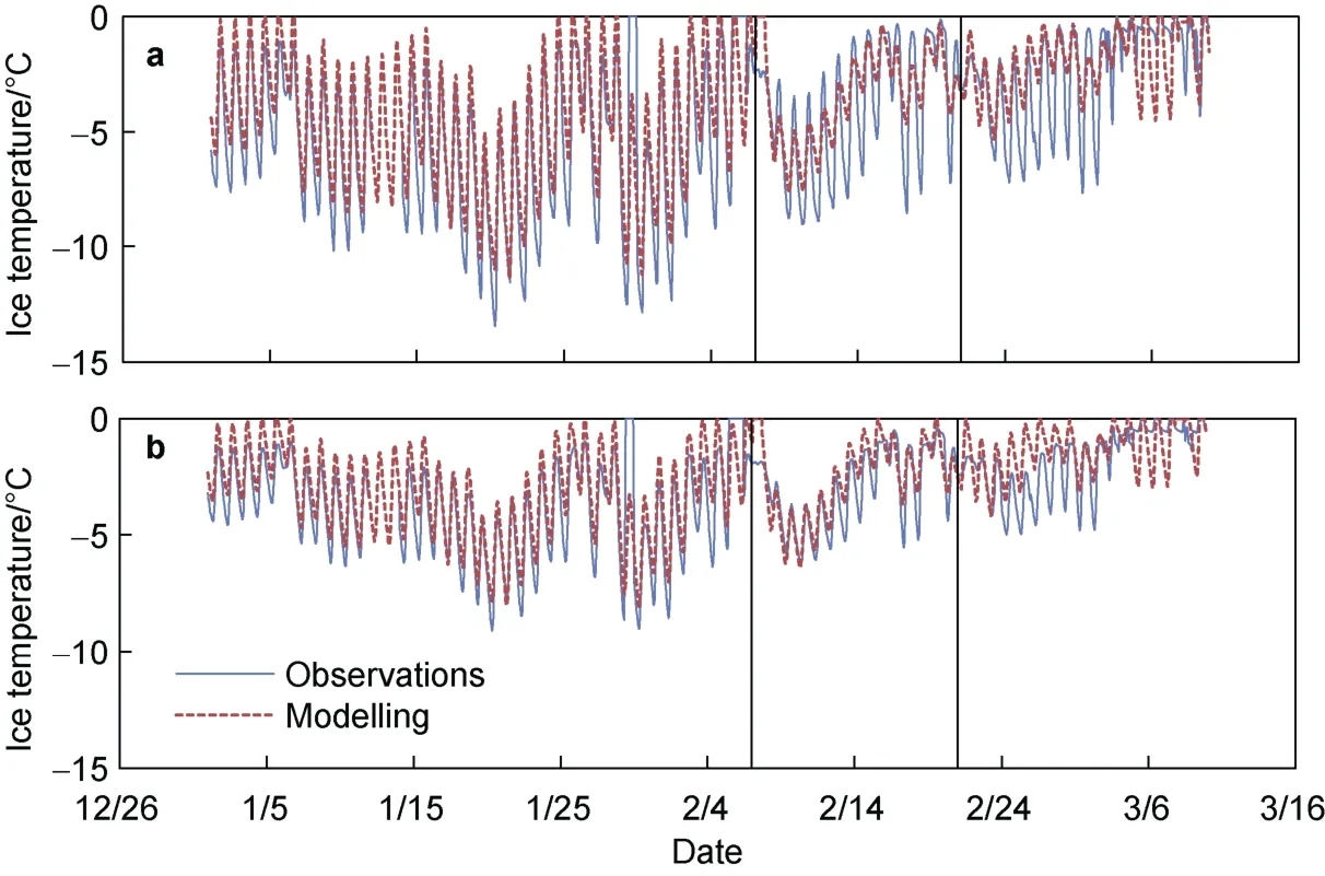
Figure 4 The modelled and measured ice temperature at 10 cm (a) and 20 cm (b) depth in winter 2017. The vertical black lines denotes the date of two snowfall events.

3.3 Vertical ice temperature profile

To further examine the accuracy of the model results, the modelled temperature profiles at 0:00, 8:00, 12:00, 16:00,and 20:00 on three typical dates (January 15, February 8,and March 5) for bare ice, snow-covered ice, and melting ice stages were selected for comparison with the measurements. The results are shown in Figure 5.

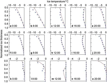
Figure 5 The modelled (lines) and observed (circles) temperature profiles at different times of day. The first row is bare ice 15 January(a-e), the second row is snow-covered ice 8 February (f-j) and the third row is melting ice 5 March (k-o).

For the bare ice period, the model results are close to the measured data with correlation coefficients higher than 0.91. The ice temperature profiles at 0:00, 8:00, and 20:00 show a linear distribution pattern and are mainly affected by the air temperature (Figures 5a, 5b, 5e). Moreover, the profiles at 12:00 and 16:00 have a “C-shape” due to the enhanced solar radiation and the increasing surface air temperature (Figures 5c, 5d). In particular, the modelled ice temperature profile at 16:00 clearly shows an increase in temperature at the thickness of 0-0.3 (Figure 5d), consistent with the results of Cheng et al. (2002), mainly due to the high temperature of the subsurface layer of the lake ice caused by solar radiation.

The snow-covered period shows similar characteristics as the bare ice case. The model agrees with the measurements, with correlation coefficients exceeding 0.94 and the average error was less than 0.07℃. The vertical pattern of the profile is also similar with the bare ice stage.The ice temperature profiles are linear at night-time(Figures 5f, 5j). During the daytime, with the increase of solar radiation, the ice temperature in the upper part increases and shows again the “C-shape” profile (Figures 5h,5i).

It is complicated during the melting stage, and most modelled results are close to the measurements, except for some points in daytime. The correlation coefficients between the model and measurements at 0:00, 8:00, and 20:00 all exceed 0.70, and the average error is less than 0.02℃ (Figures 5k, 5l, 5o). At 12:00 and 16:00, after the increase of solar radiation, there are differences in individual points in the profiles (Figures 5m, 5n). A low-temperature region in the middle of the ice layer can be found at 12:00 in both measured and model results(Figure 5m). The reason for this phenomenon is that the increase in solar radiation intensity and the increase in temperature heats up the surface ice cover, while the water body also has a heat transfer behavior for the ice bottom.Therefore, the middle depth of the ice cap is subject to both surface and surface heat transfer effects, resulting in the lowest ice temperature in the middle. However, there is no such low-temperature region in the modeled profile at 16:00(Figure 5n), 20:00 (Figure 5o), and especially at 8:00(Figure 5i). There are two main reasons for this discrepancy.On the one hand, the existence of an obvious daily freeze-melt cycle during the melting stage causes differences between the model and measurements. On the other hand, comparing with the freezing period, the physical properties of the lake ice will change in the melting period.For reasons such as the observation equipment and personnel safety, the observations during the melting phase are insufficient to correct the parameters of ice physical properties in the model.

3.4 Differences from Arctic lake ice

Lake ice in the central Asian region has its own importance and uniqueness according to the above results, and they are significantly different from others in the boreal or Arctic lakes in the high latitudes at least in the following three aspects.

First, lake ice in the boreal or Arctic regions has a longer freeze period. For example, Lake Kilpisjärvi(Leppäranta et al., 2019) in Arctic tundra and Lake Orajärvi(Cheng et al., 2014) in northern Finland both have a freezing period of about 7 months, which is significantly longer than that of the Lake Wuliangsuhai in the central Asian region. This leads to differences in the maximum ice thickness (Figure 3) and also the impact of seasonal ice cover on human life.

Secondly, the northern lake ice is always covered by a thick snow layer. Lake MacDonald (Ariano and Brown,2019) experiences high snowfall, resulting in snow ice accounting for more than 70% of the total ice thickness. It is significantly different from Lake Wuliangsuhai where snowfall is rare (Figure 4) and coagulated ice constitutes the dominant ice thickness. A thick snow cover blocks the heat exchange between atmosphere and ice, and also raises the surface albedo (Cheng et al., 2014).

Finally, less cloudy days and higher solar elevation make the lake ice in Central Asia controlled primarily by the incident solar radiation. Compared with Arctic lakes,solar radiation can easily pass through the lake ice here covered only by a thin snow layer, and then heats the water column beneath ice, which in turn increases the water-ice heat flux and warms the whole ice cover (Cao et al., 2019).

4 Summary and conclusions

The evolution of the lake ice thickness and temperature profile were simulated in the Lake Wuliangsuhai in Inner Mongolia, a typical shallow lake in the central Asian arid climate zone, by using the HIGHTSI model and the MERRA-2 data as the forcing. The simulated results were compared with and validated by the field observations conducted in winter 2017.

The simulated ice growth rate was 0.64 cm·dand-1.65 cm·dfor ice growth and melting periods of Lake Wuliangsuhai. The maximum ice thickness was 56 cm,occurring on March 3. The average ice temperature was-1.6℃ in winter 2017. The simulated ice thickness agreed well with the observations during the observation period from January 1 to March 9.

The simulated lake ice temperature also agreed with the observations, with the mean error less than 0.55℃ at the depths of 10 cm and 20 cm below the ice surface. However,the daily amplitude of the modelled ice temperature during snowfall was less than in the measurements. The main reason was the absence of the snow physical properties needed in the calculations, such as the snow density,thermal conductivity and so on. The modelled vertical ice temperature profile agreed well with observations for both the bare ice and snow-covered periods, but some differences existed in the melting period. The main reason was the lack of the measured data of lake ice physical properties of the melting period that can be modified in HIGHTSI model.

Both the HIGHTSI model and the MERRA-2 meteorological data have been proved to be feasible to simulate the seasonal evolution of the lake ice cover in Lake Wuliangsuhai. The seasonal evolution of lake ice in large time scale can be calculated in future study to investigate the difference between Lake Wuliangsuhai, a shallow lake with strong sunlight but little snow on the surface, and boreal lakes, with deep snow cover but weak sunlight in winter.

Acknowledgments

This research was supported by the National Natural Science Foundation of China (Grant nos. 51979024, 41876213,41676187), the Open Fund of State Key Laboratory of Frozen Soil Engineering (Grant no. SKLFSE201604), the Fundamental Research Funds for the Central Universities (Grant no. DUT20GJ206). Matti Leppäranta was supported by the Bilateral Exchange Programme of the Chinese Academy of Sciences and Academy of Finland (Grant no.325363). We acknowledge two anonymous reviewers, and Guest Editor Dr. Ruibo Lei for their constructive comments that have improved the manuscript significantly.