Digital Power Exchange Option Pricing under Jump-diffusion Model

LI Wen-han, ZHONG Ying, LV Gui-wen

(1- College of Mathematics and Physics, Hebei GEO University, Shijiazhuang 050031;2- Department of Mathematics and Physics, Shijiazhuang Tiedao University, Shijiazhuang 050043)

Abstract: In this paper, we propose a new option named as digital power exchange option by adding an indicator function of the ratio of the two underlying assets prices(denoted power forms) to the payoff of the power exchange option. This proposed model can be used to avoid the risk caused by the excessive price deviation of two underlying assets. Based on the above work,we obtain the explicit pricing formulas of the digital power exchange option under the jump-diffusion model by choosing the different numeraire. Finally,we take some historical data of the adjusted closing prices of two real stocks to discuss the prices of the digital power exchange option.

Keywords: digital power exchange option; avoid risk; jump-diffusion process; Esscher transform; numerical analysis

1 Introduction

Fischer[1]and Margrabe[2]proposed the definition of the exchange option, which was a more effective financial tool, to hedge against unanticipated changes with an uncertain exercise price in their pioneering work. In fact, an exchange option is a financial contract that allows the holders to receive one asset in return for paying for another at maturity. Over the past four decades,the pricing problems for the exchange option have been further considered by Gerald and Chiarella[3], Kim and Koo[4], Li et al[5]and among others.

Heynen and Kat[6]proposed another type of option called as“power option”whose payoff was a polynomial function of the underlying asset price. Esser[7]applied the technique of both change of measure and change of numeraire to several types of power options, and expanded the scope of research. As a special feature, the power option is illustrated by its payoff function. Compared to the payoff of the plain vanilla option,the underlying asset is replaced by its power function for the power option. If the exponent of the power is set to one, then the option is a plain vanilla option. Thus,the power option provides a more obvious leverage effect than the plain vanilla option in the financial market.

Blenman and Clark[8]extended both the Fischer-Margrabe exchange option and power option and presented the definition of power exchange option. This type of option provides the additional flexibility and functionality to the traditional power option and exchange option. Wang[9]and Wanget al[10]studied the pricing formula of the power exchange option as well as the power exchange option with a counter party by constructing the price processes of two underlying assets with the jump-diffusion models, respectively. In general, a more reasonable price model of the underlying asset usually consists of two sides: a continuous part and a jump-diffusion process. The jump-diffusion model was first proposed by Merton[11]. In his paper, the modeling of the asset price process is combined with a normal fluctuation process and a jump process controlled by Poisson distribution. Moreover, Kou[12], Kou and Wang[13]gave another type model—double exponential jump-diffusion process and used analytical approximation to deal with some popular path-dependent option problems.

In this present paper, we investigate a generalization of the power exchange option and further propose a new option named as the digital power exchange option (see equation (2)) by adding an indicator function of the ratio of the two underlying assets prices (denoted power forms) to the payoff of the power exchange option. Based on this structural approach, we assume that the prices of two underlying assets satisfy the jump-diffusion process under the risk-neutral measureQ. Using the Esscher transform method[14-17], we define a Radon-Nikodym derivative and introduce a new measureQ2,which is equivalent to the risk-neutral measureQ. Under the measureQ2, we take the different numeraire to obtain some pricing formulas for the digital power exchange option. In addition, we take 400 historical data of the adjusted closing prices of SBUX stock and BBY stock from November 6, 2018 to June 12, 2020 on NYSE to consider the prices of the digital power exchange option.

Following the above work, there are three contributions as follows:

(i) Adding this indicator function means adding an execution interval for the two underlying assets to the payoff of the power exchange option in [8,9]. This proposed model can be used to avoid the risk caused by the excessive price deviation of the two underlying assets;

(ii) Different from the calculating methods in[8,9], with the aid of the tool of the Esscher transform and choosing the different numeraire,we obtain the explicit formulas for the digital power exchange option;

(iii) The resulting conclusion extends the application scope of the power exchange option model in [8], and also extends the application scope of the exchange option and the power option in [6,7]. Although this extension seems to be its simplicity in the model for the payoff of the option, it may be to yield a more realistic pricing formula that only involves the digital power exchange option.

The paper is organized as follows. In section 2, we focus on the definition of the digital power exchange option and model descriptions of the dynamics for the underlying asset. In section 3, we solve the pricing problem of the digital power exchange options. In section 4, a numerical experiment for the digital power exchange option is conducted.

2 Definition and lemma

By the definition of the power exchange option in [8], at maturity, the payoff is

whereS1(t) andS2(t) are two underlying assets in the financial market, andαi,βiare some positive constants fori=1,2. Generally, we often abbreviate this payoff as

A power exchange option can be interpreted a contract as an option to exchange the power valueβ1Sα11 (T) of one asset for the power valueβ2Sα2

2 (T) of another asset at the timeT.

2.1 Definition

In this subsection,we introduce the definition of the digital power exchange option.

Definition 1Letαi> 0, βi ≥0 andKi> 0 are constants fori= 1,2. At maturity, if the payoff of an option satisfies

where [K1, K2] is the execution price interval andI{·}is an indicator function, we name this option as digital power exchange option.

Comparing with the formula (1) in [8], we add an indicator function

2.2 Model description

In order to obtain the pricing formula of the digital power exchange option with the above payoff, we first give the theoretical framework.

Let (Ω,F,{Ft},Q)(F=FT) be a complete filtered probability space, whereQis a risk-neutral probability measure. Under the measureQ, suppose that the two risky underlying assetsS1(t) andS2(t) are governed by the following stochastic differential equations

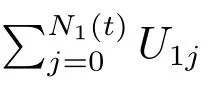
where the risk-free interest rater(t) and the volatilitiesσi(t)(i= 1,2) are all deterministic functions.W1= (W1(t))t≥0andW2= (W2(t))t≥0are two standard Brownian motions which satisfy d[W1(t),W2(t)] =ρdtwith|ρ|≤1. Fori= 1,2, the parameterλiis the jump intensity of the Poisson processNi= (Ni(t))t≥0. The sequence of random variablesUi=(Uij)j=1,2,···,Ni(t)denotes a sequence of independent and identically distributed(i.i.d)random variables and each of them is the amplitude of the jump with the density functionϕ(x). SupposeN1, N2, U1, U2andWi(i=1 or 2)are independent stochastic processes.

In order to describe the amplitude of the jump, some researchers[5,9,10,14]suppose that it follows the normal distribution and the others consider the double exponential distribution[12,13,15]. In section 2 and section 3, we do not give the specific density functionϕ(x). In section 4, conducting some numerical experiments for the digital power exchange option, we suppose thatϕ(x) is the density function of the standard normal distribution.

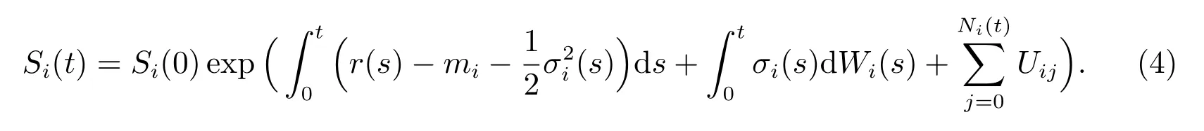
For simplicity, letmi=λiEQ(eUi −1)(i=1,2). By (3), it is easy to obtain that For the formula (4), whenNi(t)=0, it means that there is no jump risk in this model andUi0=0.

and the jump part

2.3 Esscher transform

In this subsection, we first propose an equivalent martingale measure using the random Esscher transform[16,17]and define a Radon-Nikodym derivative for the jumpdiffusion process. Thus we will generalize some conclusions to ensure that the martingale conditions hold by choosing the suitable Esscher transform parameters under the risk-neutral measure.

Lemma 1LetFYtdenote the filtration generated byY(t) for 0≤t ≤T. For

we introduce a new measureQ1equivalent toQonFYtby the Radon-Nikodym derivative

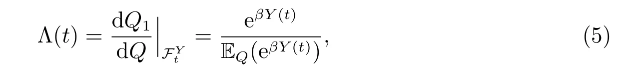
onFYt, then Λ(t) is aQ-martingale.

Under the measureQ1, the jump intensity ofN(t) and the density function ofU2become

respectively, where

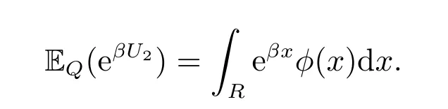
ProofFor 0≤t ≤T, note that

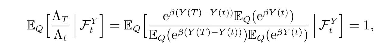
then Λtis aQ-martingale. By the following fact

we have

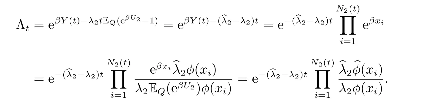
Invoking Theorem 11.6.7 in[18], we obtain that the intensity ofN2(t)and the measure density ofU2areand(x) under the measureQ1, respectively. It shows that{N(t),(U2j)}is still a stationary compound Poisson process with respect toand(x).

3 Pricing formulas of digital power exchange option

In this section, we will derive the pricing formulas of the digital power exchange option in the complete filtered space (Ω,F,{Ft}). Now, we introduce the measureQ2by

By Lemma 1, it implies that

is a martingale and the intensity ofN2(t) and the density ofU2are

under the measureQ2, respectively.

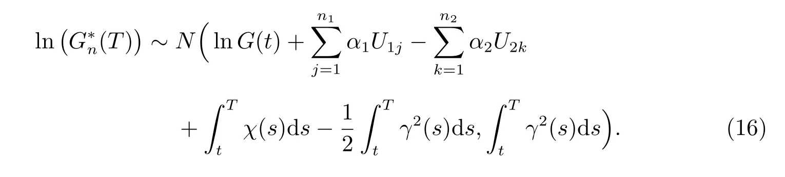
By (2), we have

and

then we can obtain that

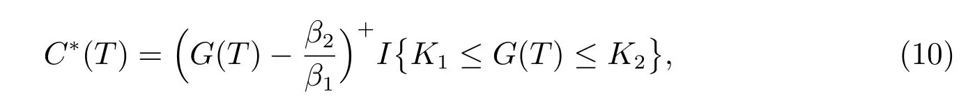
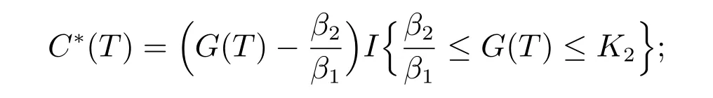
Property 1By (10), we can obtain the following conclusions:

1) If>K2, thenC∗(T)=0;

2) IfK12, then

3) If1, then

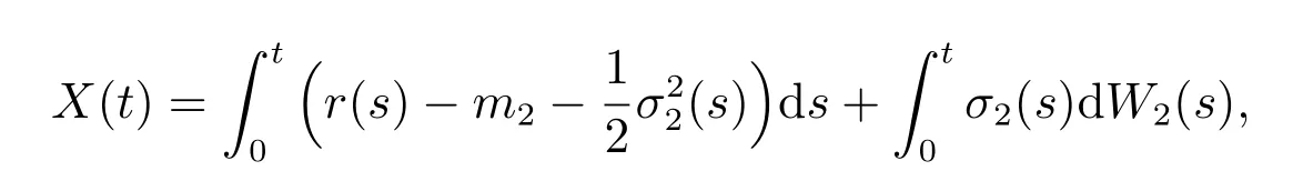
By (3), (9) and Itˆoformula, we have

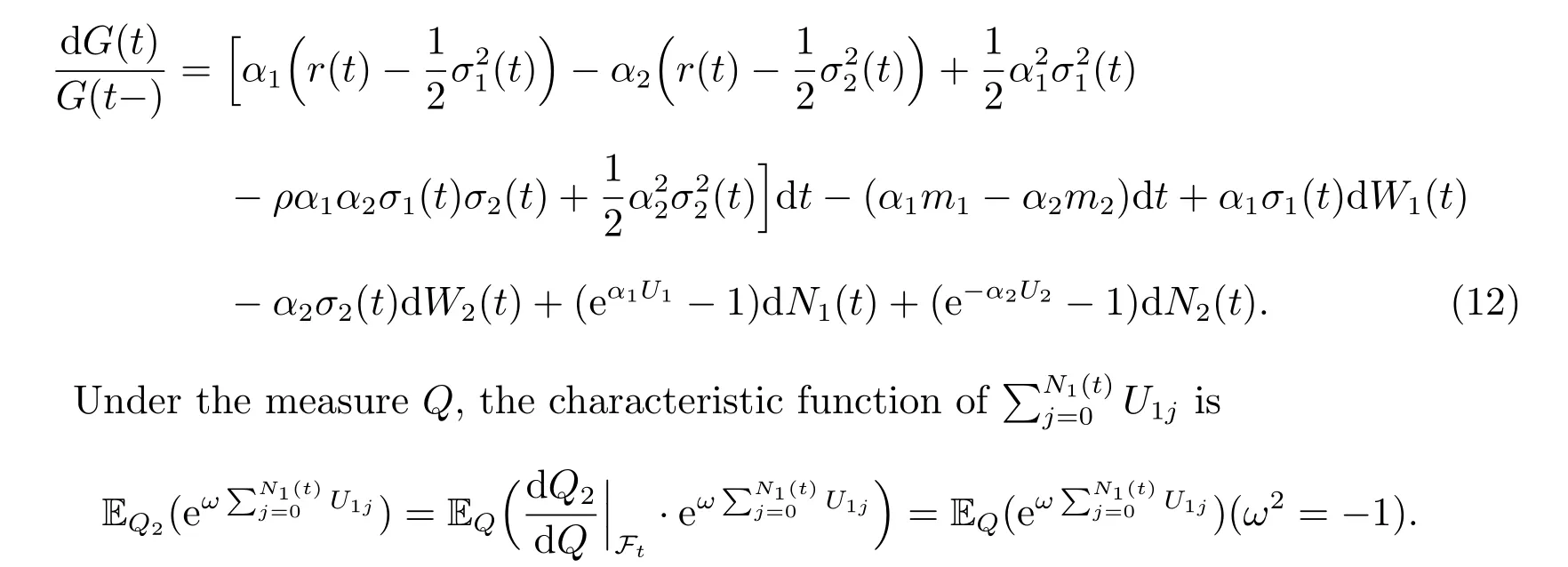
By Girsanov theorem, we obtain

are both Brownian motions under the measureQ2. Thus, (12) becomes

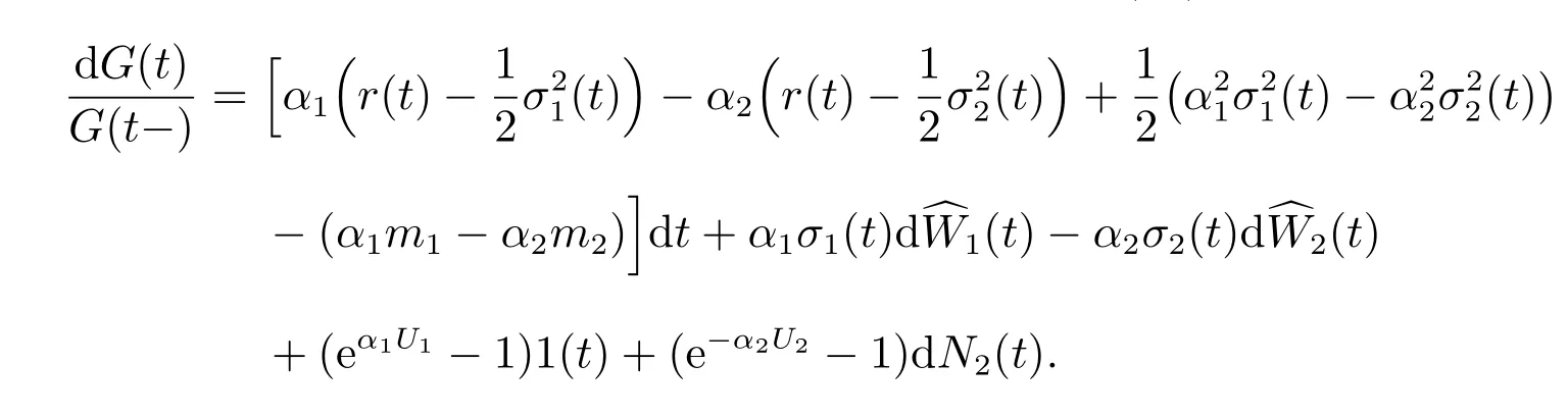
For simplicity, we rewrite the above expression as

where

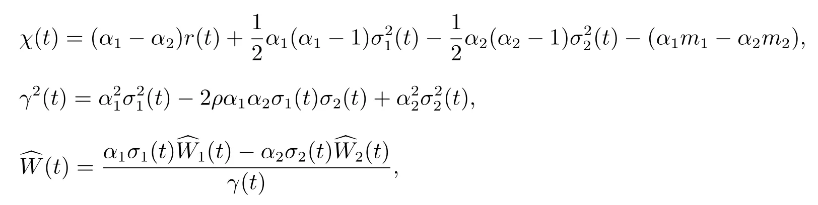
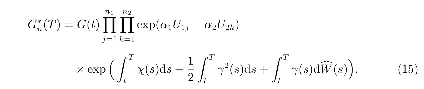
Using Dole´ans-Dade Formula, we have

whereNi(τ)=Ni(T)−Ni(t), i=1,2.

Suppose that

If take random variableUijas a common variable, then

By the above discussion, the pricing formulas of option are given by the following theorem.

Theorem 1The payoff of the digital power exchange option satisfies (2) at maturity. If the price of the assetSi(t)(i= 1,2) satisfies (3) and d[W1(t),W2(t)] =ρdtwith|ρ|≤1, then at the current timet, the digital power exchange option pricing formula denoted byC(t,T) is obtained as follows:

(i) If>K2, thenC(t,T)=0;

(ii) IfK12, then

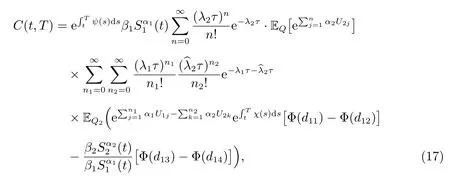
where

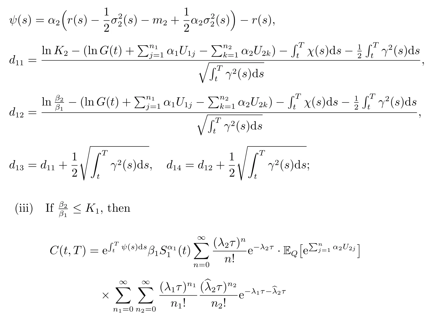
where

ProofSince the proof of (18) is similar to that of (17), we only give the proof of(17). At the current timet, the pricing formula of the digital power exchange option is given by

By (9), (10) and Property 1, we have

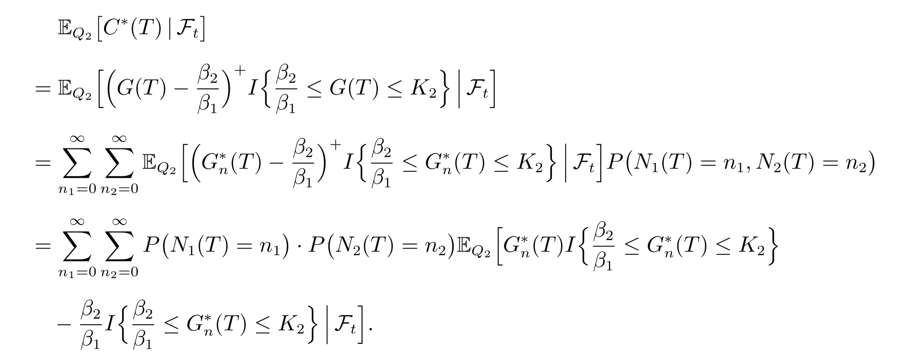
By (16), we can obtain that

Using the conditional expectation, we have

By (10), (19)–(21), we finish the proof of (17).

Remark 1From (17) in Theorem 1, some conclusions are obtained as follows:

1) Ifβ1= 1, β2∈R+, α1= 1, α2= 0, K2=∞, λ1= 0, then (17) reduces to the Black-Scholes formula for the call pricing with the strike priceβ2;

2) Ifβ1=1, β2∈R+, α1=1, α2=0, K2=∞, λ1̸=0, then (17) becomes the call pricing formula with the strike priceβ2based on jump-diffusion process;

3) Ifβ1= 1, β2∈R+, α1∈R+, α2= 0, K2=∞, λ1= 0, then (17) is the pricing formula of the power option;

4) Ifβ1= 1, β2∈R+, α1∈R+, α2= 0, K2=∞, λ1= 0, λ2̸= 0, then (17)reduces to the power option pricing formula based on jump-diffusion process;

5) Ifβ1=β2=α1=α2= 1, K2=∞, λ1=λ2= 0, then (17) reduces to the pricing formula of the standard exchange option;

6) IfK2=∞, λ1=λ2=0,then(17)reduces to the pricing formula of the power exchange option[8].

4 Numerical studies

In this section, we consider Monte Carlo simulations to illustrate the formula (17)in Theorem 1 by software programming in Matlab R2013.

In this simulation example,we try to choose two underlying assets whose prices are similar to each other based on the model of the digital power exchange option. Actually,there are many underlying assets which satisfy the above condition in the financial market. In this section, we use the adjusted closing prices of SBUX stock (S1(t)) and BBY stock (S2(t)) from November 6, 2018 to June 12, 2020 on NYSE and take 400 historical data from https://www.nyse.com/index and https://finance.yahoo.com, see Figure 1. From Figure 1, we may see that there is a similar price trend between the two stocks from December 2019 to June 2020. Thus, we further study the price of the digital power exchange option of the two stocks.

Assume that there are 250 trading days in a year. Let the random variableUi(i=1,2) follow the standard normal distributionN(0,1) under the measureQand the volatilityσi(t) be a constant. By calculation, we obtainσ1(t) =σ= 0.3685, σ2(t) =δ= 0.4732 andρ= 0.5552. It implies that the volatility of these two stocks is very large during this period. In this paper,we take January 8,2020 is the initial timet=0 and we know thatS1(0)=88.88 andS2(0)=88.65 from the historical data.

According to US Treasury Bond market in January 2020, we can know that the one-year interest rate of Treasury Bond isr(t)=0.0155. Here we takeβ1=β2=1.

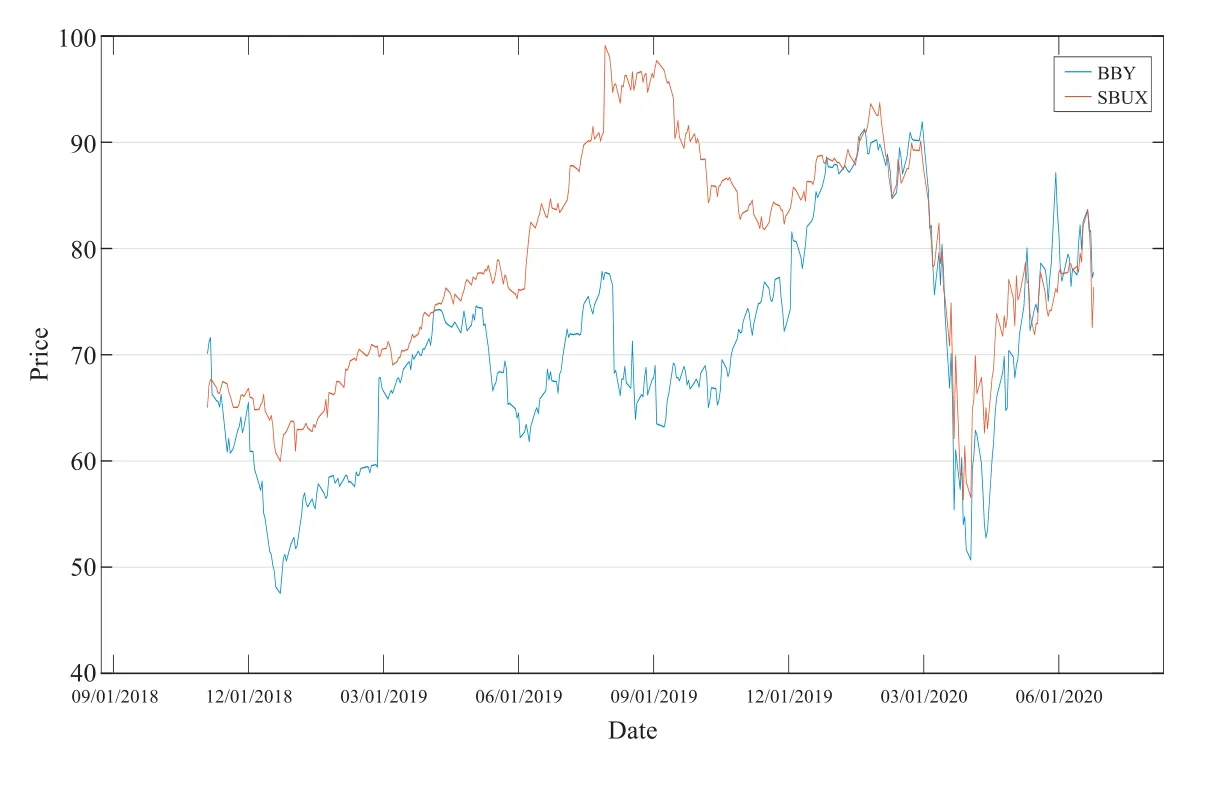
Figure 1 The trends of two stock prices

1) Suppose thatλ1=λ2=0, α1=α2=1.1 andK2=1.2,1.8,2,2.5,5,7,8, we obtain the prices of the digital power exchange option atT=1/4,1/2 and 1 in Table 1, respectively.

Table 1 Option price against K2 and T without jump process

From Table 1, it can be seen that the option price appears an increasing trend against time to maturity when the parameterK2is a fixed constant. It shows that when the parameterK2is small, the option price fluctuates greatly with the change of the parameterK2. However, ifK2is large enough, then for each fixed maturity time,the option price tends towards stability and the option price is the same as that in[8]. It also demonstrates that the option price is an increasing function with respect to the parameterK2taken a smaller value. This is just an obvious conclusion. The motivation for such an extension seems to be its simplicity in our model for the payoff of the option. However,it may be to yield a more realistic conclusion that only involves the digital power exchange option.

2) Figure 2 displays the option price for eachα1=1.15,1.2,1.25, when we takeα2=1.1, λ1=λ2=1.2 andK2=6.

It shows that the option price almost decreases as time to maturity increases in Figure 2. Note that this result differs from that in Table 1,this may be because that the jump process increases risk and affects the option value. However, it is not surprising that the option price is an increasing function with respect to the parameterα1for the fixed maturity timeTand the largerα1, the greater the influence of the option price will be. The reason is that a higher value ofα1will affect the payoff of the option strongly.

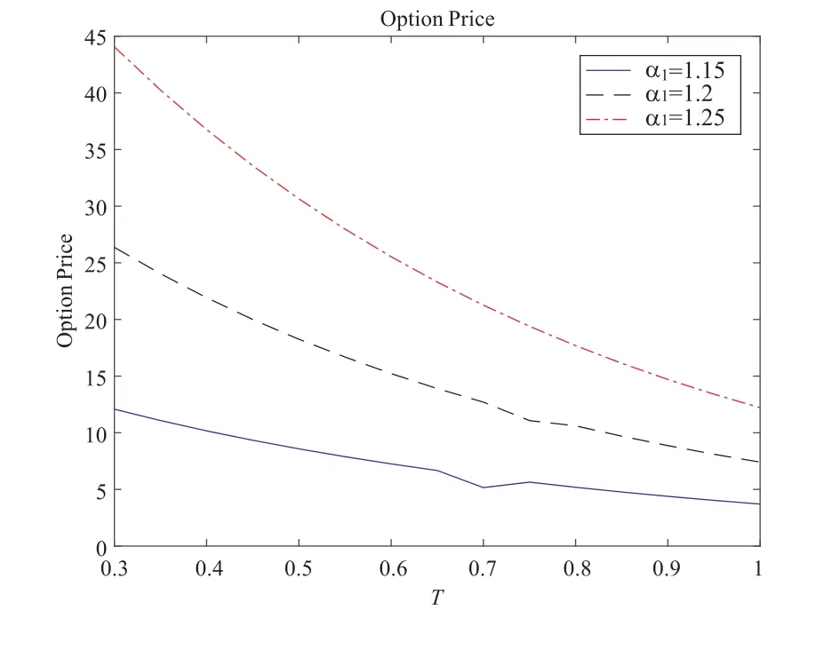
Figure 2 Option price against the maturity time

5 Conclusion

In this paper, we investigate a generalization of the power exchange option and propose the definition of the digital power exchange option by adding an execution interval about the ratio of the two underlying assets prices (denoted power forms) to the payoff of the power exchange option. The dynamics of the prices of two underlying assets are driven by Brownian process, stationary compound Poisson process and their compensation process. Under the assumption of the jump-diffusion model, we obtain the pricing formula of the digital power exchange option, and extend the application scope of the power exchange option model.