Analytic phase retrieval based on intensity measurements

1 Introduction

As a consequence,if both f and g are analytic in Ω and|f(z)|=|g(z)|,then f(z)=cg(z),where c is a constant satisfying |c| = 1. This observation shows that if we know the function value f(a) for some a ∈Ω and the amplitudes |f(z)| for all z ∈Ω, then the analytic function f(z)is uniquely determined. Without a sampled non-zero function value one can only determine an analytic function up to a unimodular multiplicative constant.

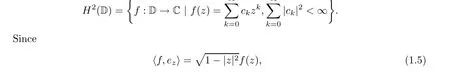
In the present paper we work in the unit disc context. For C+, the upper half complex plane, the theory and the algorithms are similar. Among the several equivalent definitions of the Hardy space H2(D),in this paper we adopt the one that is expressed in terms of the Fourier coefficients:

the 1-intensity measurements are equivalent to the |f(z)| measurements. Given the above observation on unique determination, the basic question is to compute the function values f(z)based on a sample value f(a)/=0 and the 1-intensity measurements|〈f,ez〉|.The solution of the phase retrieval problem in such a format can be achieved by using the Nevanlinna factorization Theorem involving inner and outer functions. This, as Scheme I, will be presented in Section 2.

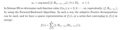
Scheme II of analytic phase retrieval, as the main part of the study, is presented in Section 3. The proposed algorithm does not involve deep analytical knowledge but only employs elementary computation based on the Gram-Schmidt orthogonalizations of certain Szeg¨o kernels.Starting from a sample value f(a) /= 0,a ∈D, the crucial technical problem is to decide f(z)at each z ∈D over two solutions of the triangle equation cos α = A so that the determined f(z) values are coherent and define an analytic function. In the computation, the intensity measurements |〈f,Baz〉| are involved. To determine f(z) we need to employ another complex number b ∈D, this being different from a and z. Correspondingly, the numerical values of the intensity measurements |〈f,Bab〉| and |〈f,Bazb〉| are involved. This algorithm is named the Forward-Backward Algorithm (FB Algorithm).

The Scheme III,as given in Section 4,is based on the selections of a1,a2,··· ,where a1=a,and is under the maximal selection principle; that is, when a1,··· ,an-1are fixed, select

2 Scheme I: Phase Retrieval Based on 1-Intensity Measurements and Nevanlinna’s Factorization Theorem

The scheme is based on the following theorem:

Theorem 2.1 ([2]) Let f(z)∈H2(D), f /≡0. Then it holds that

where C is a unimodular constant, Bf(z) is a Blaschke product made of the zeros of f, Of(z)is an outer function of f, and Sf(z) is a singular inner function of f. Except for the choice of the constant C, |C|=1, the factorization (2.1) is unique.

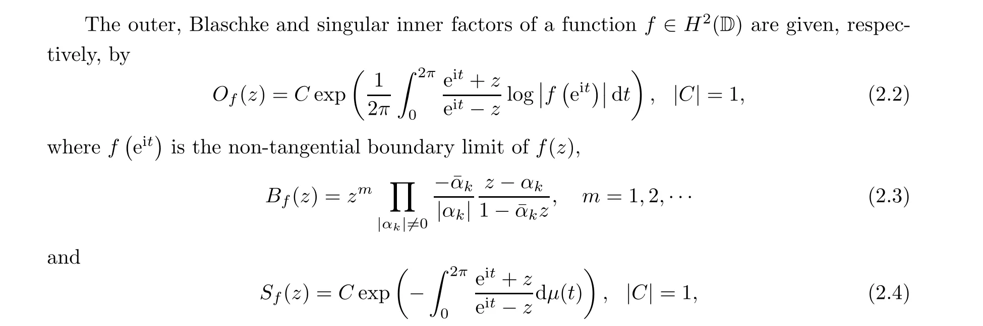
where dμ is a finite Borel measure singular to the Lebesgue measure. We note that if f is analytically extendable to an open neighbourhood of the closed unit disc,then f is continuously extendable to the boundary ∂D, and there will only be a trial singular inner function Sf=C,and inside D the function Bfwill only have finitely many zero points.

Let z ∈D be given, and let |z| ＜1. Define a Hardy space function fr(z′) = f(rz′),|z| ＜r ＜1,|z′| ＜1. We require that on ∂Drthe function f does not have zeros. The function fris analytically extended to D1rcontaining D.We have f(z)=fr(z/r)=fr(z′),z′=z/r.We assert the phase of fr(z′). Since we know |[fr(z′)]∂D|, we can first compute Ofr. Then, by solving the optimization problem

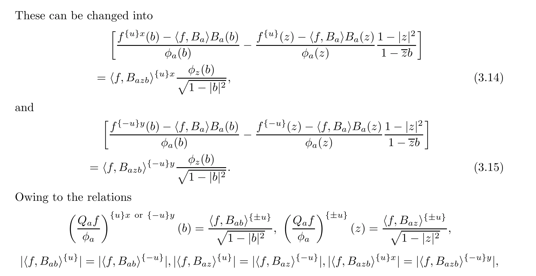
3 Scheme II: the Forward-Backward Algorithm Based on Some k-Intensity Measurements, k =1,2,3

As in the last section, we assume that a ∈D and f(a)(/= 0) are known. We assert for any z ∈D the function value of f(z). We use the orthogonal projection operators Pa1···anand Qa1···an=I-Pa1···an, where

The lemma may be extended to the cases where a1,··· ,ammay have multiplicities. In the extended cases the concept of a multiple reproducing kernel is involved ([1]).

The equation (3.8) in the complex modulus has four solutions for f(b), separated into two groups: one group corresponds to 〈f,Baz〉{+}, denoted by f{+}+(b) and f{+}-(b); the other group corresponds to 〈f,Baz〉{-}, denoted by f{-}+(b) and f{-}-(b). The ground truth value f*(b) must be among f[+](b) and f[-](b), and also among f{+}+(b),f{+}-(b),f{-}+(b) and f{-}-(b). Set

The above analysis asserts that f*(b)∈Sb∩Tb.If Sb∩Tbcontains exactly one element,then this element must be f*(b).Such a value of f*(b)is either identical with one of f{+}+(b)or f{+}-(b),or identical with one of f{-}+(b) or f{-}-(b). This implies that f*(b) is from 〈f,Baz〉{+}or〈f,Baz〉{-}, indicating that the true value f*(z) is either equal to f{+}(z) or equal to f{-}(z).With the tested examples this always happens to be the case where f{+}+(b),f{+}-(b),f{-}+(b)and f{-}-(b) are four distinct numbers, and Sb∩Tbcontains exactly one point. Theoretically,we are unable to exclude the cases where Sb∩Tbcontains two points. In this case we can sort out the one that gives the right value f*(z). A valid algorithm can be established based on the following lemma:

Lemma 3.2 Let a,z ∈D,a/=z,〈f,Ba〉/=0 and〈f,Bz〉/=0.Then for all b in a sufficiently small neighbourhood of z such that b/=a,b/=z,〈f,Bab〉/=0,〈f,Bazb〉/=0, and where b makes the opening angle between f[±](b) different from that between f{±}(z), there hold

(1) f{+}+(b),f{+}-(b),f{-}+(b) and f{-}-(b) are four distinct numbers;

(2)Sb∩Tbcontains one or two complex numbers. In both cases the right value of f(z)may be determined.

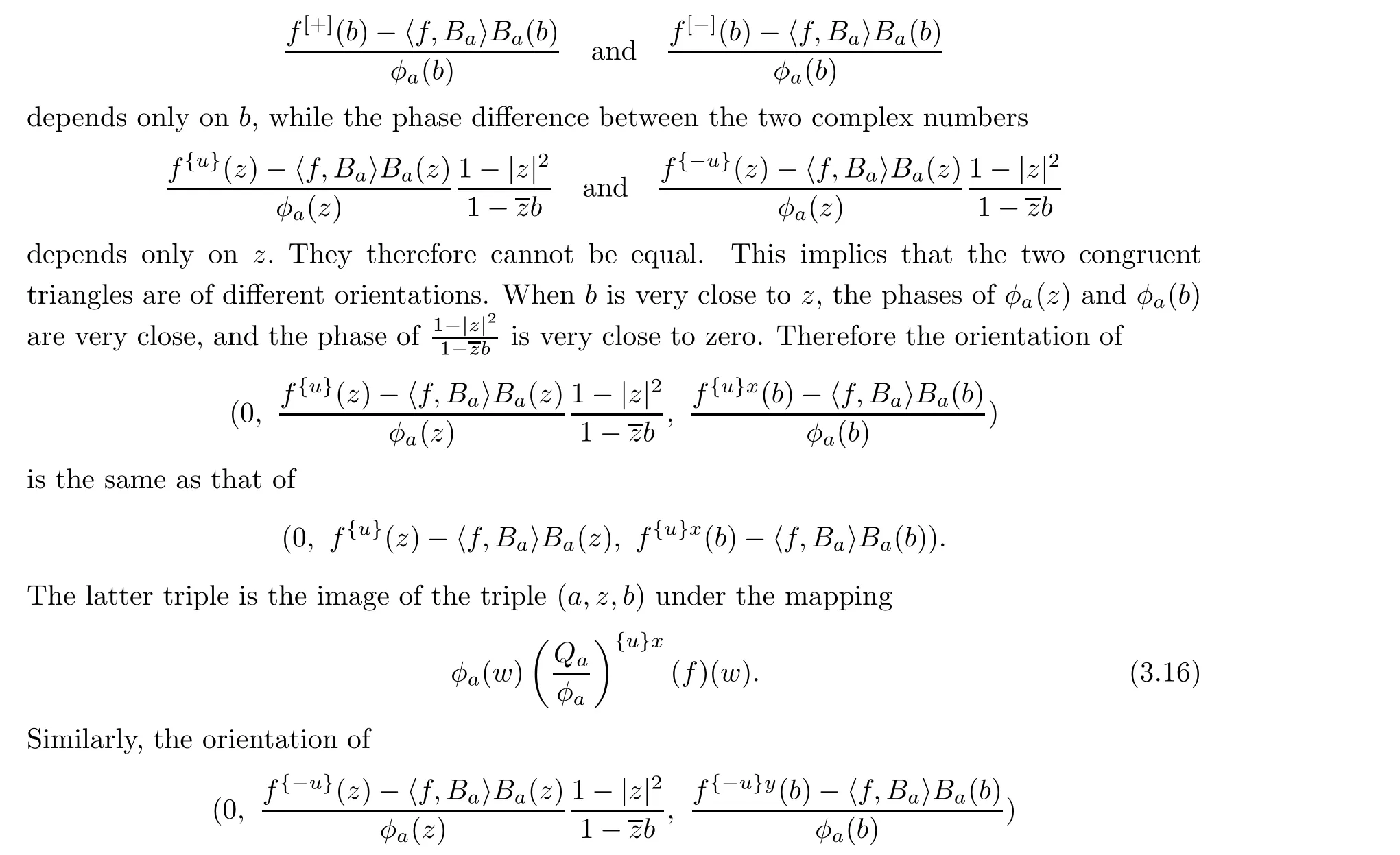
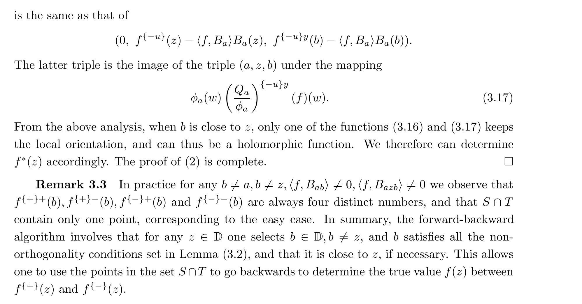
Now we prove assertion (2). Since f*(b) ∈Sb∩Tb, we have that Sb∩Tb/= Ø. If Sb∩Tbcontains only the point f*(z), then f*(b) = f{x}y(b) for a pair x and y, where each of x and y is fixed and can be + or -. In such circumstance, if x = +, then f{+}(z) = f*(z); and if x = -, then f{-}(z) = f*(z), and thus f(z) = f*(z) is determined. In the sequel this is regarded as the easy case. Next we assume that Sb∩Tbcontains two different complex numbers and accordingly derive a contradiction. In the case, Sb∩Tb= {f[+](b),f[-](b)}.Let both f[+](b) and f[-](b) be from f{+}(z). Then on one hand, the relation (3.7) implies that the solutions f[+](b) and f[-](b) are with the axis 〈f,Ba〉Ba(b). On the other hand, the solutions f{+}+(b) and f{+}-(b), which are respectively coincident with f[+](b) and f[-](b),through the relation (3.8), possess the axis 〈f,Ba〉Ba(b)-〈f,Baz〉{±}Baz(b). The two axes,therefore, are of the same direction of which one depends on only b and the other depends on b and z. For the prescribed z, a generally chosen auxiliary b rules out this coincidence from happening. The same reasoning also rules out the case where both f[+](b)and f[-](b) are from f{-}(z).So, if Sb∩Tb={f[+](b),f[-](b)},then it must be the case that f[+](b)=f{u}x(b)and f[-](b)=f{-u}y(b),where each of x,y and u can be+or-,but fixed. In the case one can show that the two triples of complex numbers, (0,f{u}(z)-〈f,Ba〉Ba(z),f{u}x(b)-〈f,Ba〉Ba(b),)and(0,f{-u}(z)-〈f,Ba〉Ba(z),f{-u}y(b)-〈f,Ba〉Ba(b)),representing two congruent triangles,are of opposite orientations. The two triples of points are respectively the images of a,z,b under the mappings

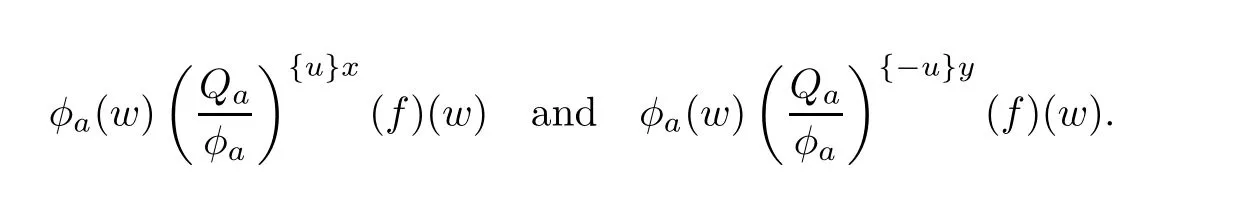
Holomorphic mappings, however, necessarily keep the local orientation. As a consequence, if b is close enough to z and a,z,b are positively oriented, the holomorphic images of a,z,b should also be positively oriented. Thus, only the triple with positive orientation corresponds to the holomorphic mapping and gives rise to the right value f(z).

To conclude the proof we need to show that(0,f{u}(z)-〈f,Ba〉Ba(z),f{u}x(b)-〈f,Ba〉Ba(b),)and (0,f{-u}(z)-〈f,Ba〉Ba(z),f{-u}y(b)-〈f,Ba〉Ba(b)) are of opposite orientations when b is sufficiently close to z. There hold the relations

we have that (3.14) and (3.15) are two solutions of the type of triangle problem described in(3.5). The two solution triangles represent two congruent triangles with different axes each having an end point adherent at the origin. We claim that the two triangles are of opposite orientations. This is based on the following geometric knowledge: if two congruent triangles have the same orientation, then the angles formed by the corresponding sides are all identical.But what we have here,however, is not the case: since f[+](b) =f{u}x(b),f[-](b) =f{-u}y(b),for the fixed a, the phase difference between

4 Scheme III: Phase Retrieval based on Sparse Representation: The AFD Type Methods

We are able to give an approximation representation formula of the phase retrieval problem. We will employ the so called adaptive Fourier decomposition (AFD, or Core AFD) or alternatively the n-best rational approximation method (Cyclic AFD). Based on a sequence of intensity measurements the AFD type methods practically give rise to approximation formulas to the solution function. We first illustrate the Core AFD method.

We still assume that we know a non-zero sample value f(a)at some point a ∈D. The AFD method involves a sequence of maximal selections of the parameters ak, k =1,2,··· to define the related Takenaka-Malmquist system. Let

converges in fast speed. Usually, for numerical purposes one needs to compute the series up to a term n. In both the infinite or finite approximation cases the error is estimated by the L2-norm of f*-f over the boundary.

Cyclic AFD offers more accurate results. Let n be fixed. When we have found, consecutively, a1,··· ,an, and accordingly formed an n-term AFD series to approximate f(z), that n-term series is usually not the optimal one over all the n-series of the same kind. To improve it, we can, for instance, let {a2,··· ,an} be an (n-1)-set, say {b1,··· ,bn-1}, and find a bn,more optimal than a1. This process of improvement is based on the fact that the orthogonal projection of f into the span of n vectors is irrelevant with the order of the vectors listed. In[4] and [7] the detailed algorithms are studied. The result of n-Cyclic AFD is of the form

where lkis the repeating number of akin the k-tuple (a1,··· ,ak). The result of n-Cyclic AFD coincides with the result of best approximation by rational functions of degree not exceeding n.

Examples of the AFD methods will be given in Section 5.

5 Experiments

We will test our methods by using two examples. One of them is taken from [3], and the other is a Blaschke product with finite zeros. In both of the examples we employ the initial value f(a) for a = 0.32-0.16i generated by a random process. With the Scheme I and II

Figure 1 Three schemes for reconstruction

Table 1 The part of function values reconstructed by Scheme I

Table 2 The part of function values reconstructed by Scheme II

Example 5.2 Let

where a1=0.51+0.22i, a2=0.83+0.1i, a3=0.39+0.13i, a4=0.25+0.64i. The initial value is f(0.32-0.16i)=0.0534+0.0377i.

By Scheme I the error r5is 0.3576×10-8.

By Scheme II the error r8is 1.0678×10-7.

By Scheme III (AFD) with an iteration number 18 the relative error is 0.0004.

The re-constructions using the three schemes are illustrated in Figure 2.

Figure 2 Three schemes for reconstruction

Table 3 The part of function values reconstructed by Scheme I

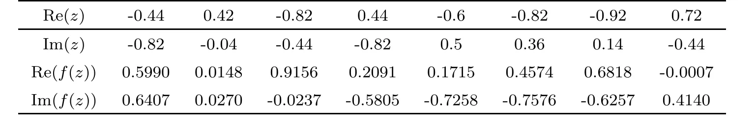
Table 4 The part of function values reconstructed by Scheme II