ENTROPICAL OPTIMAL TRANSPORT,SCHR¨ODINGER’S SYSTEM AND ALGORITHMS*

Liming WU

Institute for Advanced Study in Mathematics, Harbin’s Institute of Technology, Harbin 150001, China;Laboratoire de Math´ematiques Blaise Pascal, CNRS-UMR 6620, Universit´e Clermont-Auvergne(UCA), 63000 Clermont-Ferrand, France E-mail: Li-Ming.Wu@uca.fr

Abstract In this exposition paper we present the optimal transport problem of Monge-Amp`ere-Kantorovitch (MAK in short) and its approximative entropical regularization. Contrary to the MAK optimal transport problem,the solution of the entropical optimal transport problem is always unique, and is characterized by the Schr¨odinger system. The relationship between the Schr¨odinger system, the associated Bernstein process and the optimal transport was developed by L´eonard [32, 33] (and by Mikami [39] earlier via an h-process). We present Sinkhorn’s algorithm for solving the Schr¨odinger system and the recent results on its convergence rate. We study the gradient descent algorithm based on the dual optimal question and prove its exponential convergence, whose rate might be independent of the regularization constant. This exposition is motivated by recent applications of optimal transport to different domains such as machine learning, image processing, econometrics, astrophysics etc..

Key words entropical optimal transport; Schr¨odinger system; Sinkhorn’s algorithm; gradient descent

1 Introduction

1.1 From Monge-Amp`ere to Kantorovitch

Let μ0(dx)=f0(x)dx,μ1(dx)=f1(x)dx be two absolutely continuous probability measures on Rd. The problem of Monge-Amp`ere (Monge [41], 1781) is to find an optimal transport T :Rd→Rdsuch that

where J(T) is the Jacobian determinant of T. Intuitively T should be monotone, i.e., T =∇Φ for some convex function function Φ:Rd→R. We obtain the Monge-Amp`ere equation

Here B(S) denotes the Borel σ-field of S. A coupling Q of (μ0,μ1) is called a transport plan from μ0to μ1, and the minimiser QKis called optimal transport plan.

The advantage of Kantorovitch’s problem is that if the transport cost function c : S2→[0,+∞] is lower semi-continuous on S2, QKexists.

The disadvantage is that QKis in general not unique.

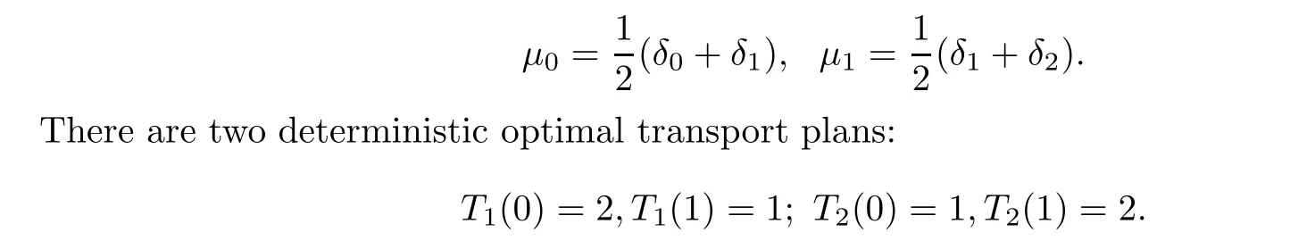
Example 1.1 S0=S1=R, c(x,y)=|x-y|,

1.2 Some recent progress in the theory

Definition 1.2 (Wasserstein metric) Let d be a metric on S, lower semi-continuous on S2, and p ∈[1,+∞). Then

is called Lp-Wasserstein distance between μ0,μ1; it is a metric on Mp1(S,d) of probability measures μ on S so that dp(x0,x) is μ(dx)-integrable (for some or any fixed point x0∈S).

A classical book on Wasserstein distance is Rachev and R¨uschendorff[46, 47].

Theorem 1.3 (Brenier [4] (1991)) Let S = Rd, c(x,y) = |x-y|2. If μ0(dx) = f0(x)dx,then Kantorovitch’s problem is equivalent to Monge’s problem: QKis the image measure of the application x →(x,Tx) of μ0for some deterministic mapping T. Moreover, T is unique,is given by T = ∇Φ for some convex function Φ, and is the solution of the Monge-Amp`ere equation which is unique up to a difference of a constant.

The progress made in the study of the optimal transport problem in the last thirty years has been spectacular. Otto and Villani, along with their collaborators,developed a differential theory on M21(Rd) and showed that many PDEs are the gradient flow of some entropy or energy functional. Lott-Villani and Sturm built a geometric theory on M21(M)for a Riemannian manifold or Alexandrov-Gromov’s space M. Figalli used optimal transport to solve some PDEs.The reader is referred to the books of Villani [55, 56].

1.3 Applications

The optimal transport plan itself(either as a coupling QKor a Monge map T when it exists)has recently found many applications in data science, and in particular in image processing. It has, for instance, been used for

(1) contrast equalization, cf. Delon [15] (2004);

(2) texture synthesis, cf. Gutierrez et al. [26] (2017);

(3) image matching, see Zhu et al. [59] (2007), Museyko et al. [42] (2009), Li et al. [34](2013), Wang et al. [58] (2013);

(4) image fusion, cf. Courty et al. [9] (2016);

(5) medical imaging, cf. Wang et al. [57] (2011);

(6) shape registration,see Makihara and Yagi [37] (2010),Lai and Zhao [31] (2017), Su et al. [54] (2015);

(7) image watermarking, cf. Mathon et al. [38] (2014);

(8) for reconstructing the early universe in astrophysics,cf. Frisch et al. [21] (2002);

(9) in economics, to interpret matching data, cf. Galichon [23] (2016).

(10) to perform sampling, cf. Reich [48] (2013),Oliver [43] (2014)and Bayesian inference,cf. Kim et al. [28] (2013), El Moselhy and Marzouk [17] (2012).

For a review of applications of optimal transport to signal processing and machine learning,see Kolouri et al. [29]. For optimal transport in applied mathematics, see Santambrogio [51];in economics see Erlander [18], Erlander and Stewart [18].

1.4 How to compute the optimal transport?

Kantorovitch’s optimal transport plan is a problem of linear progamming(Dantzig[13,14]).For computation purposes we suppose that μ0(resp. μ1) is supported by a finite subset S0={x1,··· ,xm} (resp. S1={y1,··· ,yj}) in S. Then C(μ0,μ1) is a convex simplex, the cost of a transport plan Q

The set of extreme points of C(μ0,μ1) is identified as all permutations on {1,··· ,n}, i.e.,any extreme transport plan Q=(qij) is characterized by

for some permutation σ. Hence there are n!extreme points for this optimal assignment problem.

2 Entropy Regularization of Kantorovitch’s Optimal Transport: the Finite Case

and (μ0⊗～A)(xi,yj)=μ0(i)～aij.

The minimization of relative entropy with given marginal distributions or with general constraints was studied by Csiszar [11]. The entropy optimisation (2.1) is closely related to the optimal transport by the following simple computation: letting qij= Q(xi,yj), Q(j|i) =qij/μ0(i), which is the conditional probability of yjgiven xiunder Q, we have

for any Kantorovitch optimal transport plan QK.

QEis called entropical optimal transport plan.

Proof As the entropy functional H(Q|μ0⊗～A) is strictly convex and inf-compact, then its minimiser QE=(qEij) on the convex and compact set C(μ0,μ1) exists and it is unique.

Exchanging the roles of μ0and μ1, we obtain (2.4). For the last claim, see Peyr´e and Cuturi[44, Sect.4].□

Remark 2.2 The key new idea of using ～A (or A) in (2.2) for relating the maximum entropy problem to optimal transport comes from L´eonard[32,33](earlier,Mikami[39]related the h-process to optimal transport), see the recent monographs [40, 44] for the history and a rich list of references. Our presentation beginning with (2.1) is inspired by [10, 32, 33].

3 Schr¨odinger’s System

From now on we assume always that cij:=c(xi,yj)＜+∞,μ0(i)μ1(j)＞0 for all (i,j).

Theorem 3.1 (a) Q ∈C(μ0,μ1) is the minimiser QEof (2.1) iffthere are a pair of everywhere positive functions ψ,φ on S0= {xi,i = 1,··· ,m},S1= {yj,j = 1,··· ,n} such that

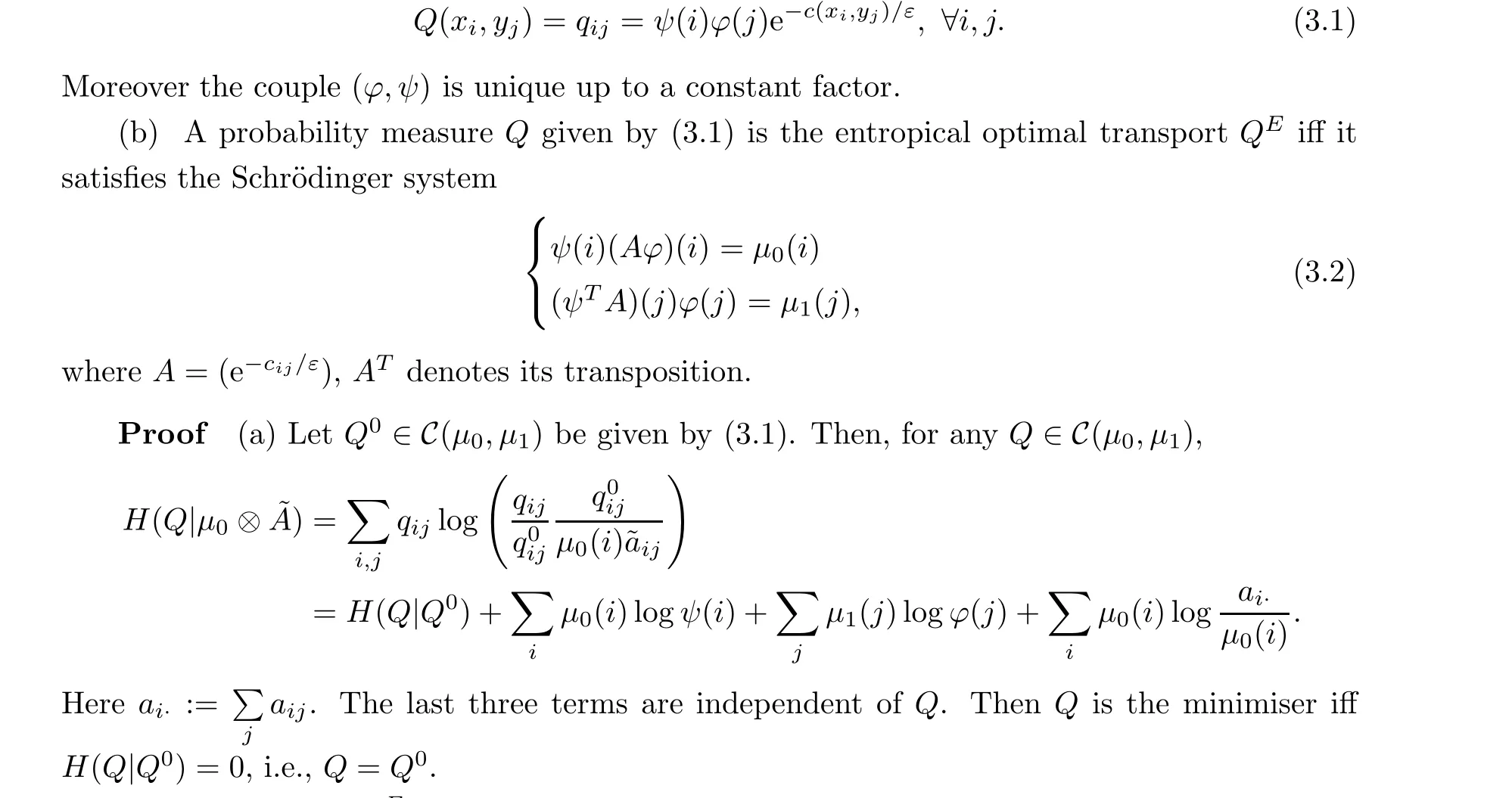
The inverse that QEmust be of form (3.1) is the Gibbs principle, proven by Csiszar [11](valid in the actual finite case).

(b) This is obvious from part (a), because Q given by (3.1) belongs to C(μ0,μ1) iff(ψ,φ)satisfies the Schr¨odinger system.

Remark 3.2 The system of equations (3.2) for a given reference kernel K instead of ～aijwas introduced by Schr¨odinger [52] (1931). The existence and the uniqueness of a solution of the Schr¨odinger system was proved first by Beurling [2] (1960). Later, the Schr¨odinger system related to the maximum entropy principle and to Bernstein processes was studied by Cruzeiro et al. [10]. Its relationship with optimal transport was found by Mikami [39] via the h-process and L´eonard [32, 33] by means of the maximum entropy principle.

Remark 3.3 The Gibbs principle for the mimimiser QEof the relative entropy with the two given marginal distributions was first investigated by Csiszar [11], but when the reference measure μ0⊗～A becomes general(in the general state space case),part(a)above may be wrong.For this subtle question see L´eonard [32, 33] and the references therein.

4 Sinkhorn’s Algorithm

In what follows, for simplification of notation, we will identify xias i, and yjas j. For instance, f(i)= f(xi), g(j)= g(yj), cij=c(xi,yj). Given an everywhere positive function φ0on S1, Sinkhorn’s algorithm goes as follows:

The proof of the convergence of this algorithm is attributed to Sinkhorn [53] (1964). This algorithm was later extended in infinite dimensions by R¨uschendorf [49] (1995). Sinkhorn’s algorithm has received renewed attention in econometrics after Galichon and Salani´e[22](2010),and in data science(including machine learning,vision,graphics and imaging)after Cuturi[12](2013),who showed that Sinkhorn’s algorithm provides an efficient and scalable approximation to optimal transport, thanks to seamless parallelization when solving several optimal transport problems simultaneously (notably on GPUs).

A crucial tool for the analysis of the convergence rate of Sinkhorn’s algorithm is the Hilbert metric on everywhere positive functions up to a constant factor. For two positive functions u,v ＞0 on S1, u ～v if u = cv for some constant c. The Hilbert metric on (0,+∞)n/ ～is defined by

In other words, a totally positive matrix K is always a contraction in the Hilbert metric(as λ(K)＜1).

Theorem 4.2 (a) (Sinkhorn [53] (1964)) For Sinkhorn’s algorithm, (ψk,φk) →(ψ,φ)in dH, a solution of the Schr¨odinger system (3.2).

(b)(Franklin and Lorenz[20](1989))based on Theorem 4.1) For Qk(i,j)=ψk(i)aijφk(j)(k ≥1),

Remark 4.3 If ε ＞0 is very small, as λ(A) = 1-O(e-C/ε), the theoretical geometric convergence rate in Theorem 4.2(b) is bad; as is emphasized in [44, 45], the convergence of Sinkhorn’s algorithm deteriorates when ε is too small in numerical practice.

Remark 4.4 For more recent progress on Sinkhorn’s algorithm for solving Schr¨odinger’s system, see Di Marino and Gerolin [16].

5 Dual Problem: A Gradient Descent Algorithm

As the convergence of Sinkhorn’s algorithm deteriorates when the regularization parameter ε becomes small, it is natural to check other algorithms. See Peyr´e and Cuturi [44, 45] for different refinements and generalizations of Sinkhorn’s algorithm. The purpose of this section is to propose the gradient descent algorithm for the dual optimisation problem, to prove its exponential convergence with a rate λ in terms of some Poincar´e inequality(Theorem 5.2),and to show that λ may be independent of ε ∈(0,1) in some particular case (Corollary 5.5).

The dual problem of (2.3) is ([44, Section 4])

We see that ∇(f,g)Φ(f,g)=0 iff(ψ,φ)=(ef/ε,eg/ε) satisfies Schr¨odinger’s system (3.2). Thus we obtain, by Theorem 3.1,

Then the maximiser (f*,g*) of (5.2) exists and is unique. This also gives another proof of the existence and the uniqueness of Schr¨odinger’s system in Theorem 3.1 in the finite case.

Step 2 (Bipartite graph and Poincar´e inequality) We want to get some quantitative lower bound of ∇2V on H. For this purpose, consider the bipartite graph W = {1,··· ,m}∪{1′,··· ,n′} with the set E of (non-oriented) edges {i,j′}, i = 1,··· ,m; j = 1,··· ,n (we add a prime to j to distinguish xiand yjeven when they are at the same position). Introduce the function h:W →R associated with (a,b)∈Rm×Rnby

for all t ≥t0. We get (5.8), again by Gronwall’s inequality.□

Remark 5.4 The spectral gap λ1(f,g) for the Dirichlet form E(f,g)defined in (5.10) is a well-studied object in graph theory (Chung [8], Ma et al. [36], Cheng et al. [7]). The first rough lower bound can be obtained in the following way: first,

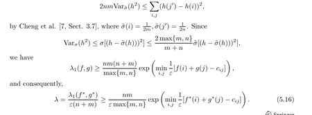
When ε ＞0 is too small,this might be bad,as with the estimate in Theorem 4.2 for Sinkhorn’s algorithm. However we can do much better.

Corollary 5.5 Assume that the bipartite graph W = {i,j′|1 ≤i ≤m,1 ≤j ≤n}equipped with the edges subset

which yields the desired result.

Remark 5.6 When the optimal transport plan QKfor Kantorovitch’s problem is unique such that W, equipped with the edges set E0:= {{i,j′};QK(xi,yj) ＞0} is connected, then(W,E0) is a tree (because QKmust be an extreme point of C(μ0,μ1)). For this tree case, see W. Liu et al. [35] for a sharp estimate of the spectral gap λ(E0).

The gradient descent or stochastic gradient descent algorithms(if m is very big)for finding the minimiser of-Ψ(g)were studied in Genevay et al. [24];see also Peyr´e-Cuturi[44,45]. However whether the gradient descent algorithm for finding the minimiser of -Ψ(g) is exponentially convergent with a quantifiable rate is still an unsolved question.

This, indeed, is also our main motivation to study directly the gradient descent algorithm(5.4) and to show its exponential convergence in Theorem 5.2. The bipartite graph structure and the Poincar´e inequality used for proving Theorem 5.2 show that the unsolved question stated above for finding the maximiser of Ψ(g) is a quite delicate question, worthy of being studied further.

To the memory of Professor Yu Jiarong I was a young teacher-researcher at the Sino-French Center of Mathematics in Wuhan University during 1987-1993 when Prof. Yu presided there. His encouragement and support were always strong and precious. His sincerity,kindness and warmness towards the people he worked with and to mathematics are in our mind forever.

Acknowledgements I am grateful to Christian L´eonard for conversations on this fascinating subject, to Wei Liu and Yuling Jiao of Wuhan University for the communication of several references, to Xiangdong Li for the kind invitation to the conference on optimal transport held on May 2021 at AMSS, Chinese Academy of Sciences, where the material of this exposition paper was reported.