Numerical study of morphological characteristics of rotational natural supercavitation by rotational supercavitating evaporator with optimized blade shape ＊

Zhi-ying Zheng , Qian Li Lu Wang , Li-ming Yao , Wei-hua Cai Hui Li Feng-chen Li

1. School of Energy Science and Engineering, Harbin Institute of Technology, Harbin 150001, China

2.School of Civil Engineering, Harbin Institute of Technology, Harbin 150090, China

3.Department of Nuclear Engineering, Kyoto University, Kyoto, Japan

4. College of Aerospace and Civil Engineering, Harbin Engineering University, Harbin 150001, China

5.Institute of Advanced Technology, Heilongjiang Academy of Sciences, Harbin 150020, China

6.Sino-French Institute of Nuclear Engineering and Technology, Sun Yat-Sen University, Zhuhai 519082, China

Abstract: In view of the supercavitation effect, a novel device named the rotational supercavitating evaporator (RSCE) has been designed for the desalination.In order to improve the blade shape of the rotational cavitator in the RSCE for the performance optimization, the blade shapes of different sizes are designed by utilizing the improved calculation method for the blade shape and the validated empirical formulae based on previous two-dimensional numerical simulations, from which the optimized blade shape with the wedge angle of 45° and the design speed of 5 000 r/min is selected.The estimation method for the desalination performance parameters is developed to validate the feasibility of the utilization of the results obtained by the two-dimensional numerical simulations in the design of the three-dimensional blade shape.Three-dimensional numerical simulations are then conducted for the supercavitating flows around the rotational cavitator with the optimized blade shape at different rotational speeds to obtain the morphological characteristics of the rotational natural supercavitation.The results show that the profile of the supercavity tail is concaved toward the inside of the supercavity due to the re-entrant jet.The empirical formulae for estimating the supercavity size with consideration of the rotation are obtained by fitting the data, with the exponents different from those obtained by the previous two-dimensional numerical simulations.The influences of the rotation on the morphological characteristics are analyzed from the perspectives of the tip and hub vortices and the interaction between the supercavity tail and the blade.Further numerical simulation of the supercavitating flow around the rotational cavitator made up by the blades with exit edge of uniform thickness illustrate that the morphological characteristics are also affected by the blade shape.

Key words: Rotational natural supercavitation, morphological characteristics, blade shape, computational fluid dynamics (CFD)numerical simulation, rotational supercavitating evaporator

Introduction

As the most effective and promising solution to the increasingly severe fresh water shortage throughout the world, the seawater desalination has attracted much attention of both scientific and industrial fields,and inspires the development of both conventional and modern desalination technologies.The current major large-scale industrial desalination technologies include the multi-stage flash (MSF), the multiple effect distillation (MED) and the reverse osmosis(RO).The first two are thermal methods based on the principle that the fresh water is acquired by the condensation of the vapor from the heated raw water.The RO is a membrane method, in which the osmotic pressure across a semipermeable membrane is resisted to drive the diffusion of water molecules through the membrane.However, the existence of solid walls in the MSF and the MED causes the problems of scaling and fouling, resulting in the decrease of the heat transfer coefficient, while a rigorous pre-treatment is indispensable in the RO for avoiding the fouling formation and the low recovery factor.

To overcome the above-mentioned shortcomings of the main conventional desalination methods, a novel device named the rotational supercavitating evaporator (RSCE) has been proposed and designed by utilizing the characteristics of the hydrodynamic supercavitation effect[1-4], i.e., a large energy intensity and a large heat-mass transfer rate at the steam-water interface and no formation of scaling.This method is similar to a thermal method, the phase change occurs in the desalination process, with a difference in the fact that the phase change is caused by the cavitation,i.e., the vaporization of the liquid and the abrupt expansion of nuclei inside the liquid into obvious bubbles by the decrease of the local pressure under roughly constant temperature.Supercavitation is the most intense level of the cavitation generated at a low characteristic pressure or a large characteristic velocity.

Most of the studies of the application of the hydrodynamic cavitation in the desalination were conducted by Russian researchers, with a scarcity of the relevant published literature.In 1984 Machinski introduced a stationary conical supercavitating evaporator into the desalination, with the ability to create a relatively stable supercavity and be connected to a vacuum system for the steam extraction[5].However, the entire system includes multiple cascading evaporators, and a continuous high-volume recirculation of the subcooled hot source water through the system is required in its industrial applications for the desalination.This scheme is metal-intensive and the ratio of the supercavity volume to the water bulk volume is very small, and an energy-intensive pump recirculation system is also required.Combining the electromagnetic treatment with the supercavitation, the scientific and technical center “TJEROS-MIFI” in Russia designed and manufactured a commercial cavitating desalination device “WATERFALL-1200” with a productivity of 1 200 m3/d[6].This device consumes the electrical energy up to 3 kWh for unit volume of fresh water and ensures a rejection rate better than 99% under the operation of the source water with total dissolved solids (TDS) up to 65 000 mg/L, which is significantly competitive with the current major large-scale industrial desalination technologies (The energy consumptions of MSF, MED and RO can be found in Ref.[7]).Langenecker and Zeilinger[8-10]developed a hydrodynamic cavitation system for the desalination,in which instead of the generation of the supercavity for the steam extraction within, the sonochemistry effect caused by the collapse of the bubbles was utilized to break the mechanical bonds of the metallic salts (e.g., sodium chloride) to form new combinations with the surface-active particles added into the raw water.Ultimately, the desalination can be achieved by removing these particles through a simple filtration.The prototype had an energy consumption amounting to 1.1 kWh/m3[8-9], and the raw water of 1 400 mg/L of the TDS could be desalinated into fresh water of 400 mg/L of the TDS[10].Besides the hydrodynamic cavitation, the acoustic cavitation was also applied for the desalination in the form of the ultrasonic atomization[11-12].

Recently, the RSCE was put forward by Likhachev et al.[1-3,5]and fabricated for the desalination or the purification of polluted water.The first attempt to conduct relatively complete performance test of the RSCE includes the design of the blade shape, the manufacture of the rotational cavitator, the establishment of the test system and the experimental test and analysis.In the first place[2], the shape of the RSCE under the design condition at the rotational speed of 10 000 r/min was mathematically determined by using empirical equations in which the drag coefficient and the empirical coefficient were obtained through experiments for the plane-parallel supercavitating flow around the wedge-shaped cavitator.The geometrical characteristics of the supercavity generated by the RSCE at the rotational speed of 10 000 r/min were then obtained through the numerical simulation, and the location of the area suitable for the steam extraction was also determined according to the inner structure of the supercavity.However, under the real experimental conditions, the highest rotational speed at which two separated supercavities occupying most of the space between the blades were generated behind two blades was 5 430 r/min instead of 10 000 r/min.Moreover, the cavitator with the same profile but only a quarter of the original dimension (400 mm in diameter), i.e., 130 mm in diameter, was chosen for the experiment due to the limitation of the motor power[5].The multiple factor extremal experiments were conducted with the Box-Wilson’s method and the regression analysis for the water flow at the temperature of around 22°C-30°C and the atmospheric pressure[3].The statistically valid regression equations were formulated to accurately reproduce the supercavity length at different radial locations along the impeller blade during the rotational supercavitation in cold water for the combinations of the steam extraction rates of 5.2 m3/h-8.2 m3/h and the rotational speeds of 3 950 r/min -5 430 r/min.

In light of the above-mentioned problems in the first attempt to systematically investigate the performance of the RSCE, further studies of the hydrodynamic characteristics of the RSCE and the influencing factors should be conducted to optimize its desalination performance.The core component of the RSCE is a rotational cavitator made of two blades of wedge-shaped cross section and the exit edge of alternative thickness.It is used for the formation of the supercavitation and the production of steam.Therefore, the hydrodynamic characteristics of the three-dimensional blade shape are of great importance for the performance of the RSCE.This paper focuses on the morphological characteristics of the supercavity generated by the rotational supercavitating evaporator of optimized blade shape.

1.Design and modelling of three-dimensional blade shape

1.1 Improvement and design of three-dimensional blade shape

All empirical formulae for the dimensionless supercavity length as a function of the cavitation number were obtained and validated by the existing experimental results obtained in our previous work[13],based on which the blade shape of the RSCE can be determined for various wedge angles (2αin Fig.1 of Ref.[13]) and rotational speeds (defined as the design speeddω).Practically, the three-dimensional blade shape is determined by fixed wedge angles and alternative thicknesses of the exit edge (2hin Fig.1 of Ref.[13]) at different radii, while the thickness of the exit edge is determined by the comparison between the supercavity lengthLand the arc lengthp(the arc from the exit edge of the blade to the entrance edge of the next blade, i.e., the arc BC′ in Fig.1) at the corresponding radius.

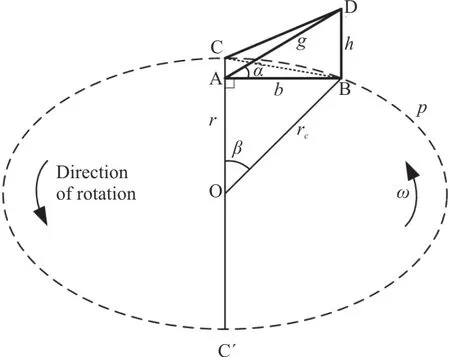
Fig.1 Schematic diagram of the improved calculation method for the blade shape

However, the values of 2αat different radii in the original calculation method for the blade shape(Fig.3 in Ref.[2]) are not exactly equal to the desired wedge angle.Moreover, the deviation would increase with the decrease of the radiusr.To address this issue, an improved method is proposed, as shown in Fig.1, in which the length of the supercavityLis obtained by replacing the radius at the entrance edgerwith the radius at the exit edgecr.Note that only half of the isosceles triangular cross section of the blade model is given in Fig.1 for a clear depiction.Detailed algorithm for the thickness of the exit edge is illustrated in Fig.2, and as follows:

(1) Specifying the ambient pressurep∞, the density of the liquidρl, the saturated vapor pressurepvcorresponding to the ambient pressure, the half of the wedge angleα, the periphery radius of the bladeR, and the design speedωd.

(2) Equally dividing the entrance edge of the blade (OC in Fig.1) intoNsegments, and initializing the half-thickness of the exit edgeh(i) atr(i) (i=1,2,… ,N, andr(i)=0 fori=0).

(3) Calculatingb(i),β(i),rc(i),p(i), based on the geometric conditions (herein,p=(360/n-β)πrc/180, wherenis the number of blades), and then the linear speedv(i)(v=ωdr c), andσ(i) according to the definition of the cavitation number (σ=2(p∞-pv)/ρlv2).Calculating the supercavity lengthL(i) based on the empirical formulae obtained in our previous work[13].

(4) Iterating forh(i) atr(i) by increasingh(i) by an increment Δhuntil the conditionL(i) ＜p(i) cannot be satisfied, and then continuing the calculation for the nextiuntil the periphery radius of the blader(N)=Ris reached.

Fig.2 Algorithm for obtaining the blade shape (i.e., half-thickness of the blade’s exit edge h)

(5) Obtaining the desired parameters:h(i),β(i),rc(i) andL(i) atr(i).

The blade shape in this study is calculated based on the following input parameters:p∞=101325 Pa,ρl=997 kg/m3,pv=3169.9 Pa,R=0.2 m,n=2,N=20 and Δh=1× 10-5m.Herein, the values ofρlandpvare set in line with the international standard for the thermodynamic properties of water and steam IAPWS95[14]at 25°C.

According to the proposed calculation method,there exists a corresponding blade shape for each wedge angle 2αand design speedωdas mentioned above.The design speedsωdranging from 1 000 r/min to 5 000 r/min with an increment of 1 000 r/min are taken into consideration, while the wedge angle 2αis varied from 30° to 150°, as in the previous work[13].The variations of the half-thickness of the exit edgehagainstrfor different wedge angles at different design speeds and for different design speeds at different wedge angles are shown in Figs.3, 4, respectively.It is shown in Fig.3 thathdecreases with the increase ofrfor each blade shape.The difference between the half-thicknesses of the exit edges at the blade root and at the blade tip increases with the increase of the wedge angle for the same design speed.Thus, in view of the size of the shaft(due to the need of a larger shaft length for a certain shaft diameter or a larger shaft diameter for a certain shaft length at larger wedge angles) and the blade length (because of the requirement for the mechanical strength at a larger radius wherehis too small), the blade shape with a smaller wedge angle is more suitable.On the other hand,hfor eachrdecreases with the increase of the design speed for the same wedge angle, as shown in Fig.4.Hence, the blade shape designed for a relatively high design speed is selected on account of the sizes of the shaft and the blade.With adequate consideration of the blade’s mechanical strength,h=1 mm is adopted in the design of the blade shape.Ultimately, the optimized blade with 2α=45° andωd=5000 r/min is designed.Its model is schematically shown in Fig.11(a).The detailed half-thicknesses of the exit edge at different radii are shown in Table 1.The shaft diameterd0and the diameterdof this blade are 70 mm and 200 mm, respectively.

1.2 Estimation of desalination performance parameters

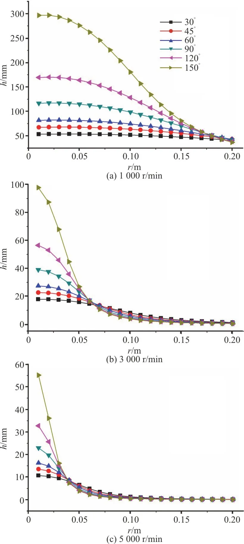
Fig.3 (Color online) Variations of half-thickness of the exit edge h against the radius r for different wedge angles at different design speeds

Since the empirical formulae for the supercavity length adopted in the design of the three-dimensional blade shape are obtained by two-dimensional numerical simulations, its feasibility needs to be verified.For the verification, the desalination performance parameters of the RSCE are estimated by utilizing the results of the two-dimensional numerical simulations,and then compared with the results of the three-dimensional numerical simulations.According to the working principle of the RSCE and the definition of the energy consumption of the desalination technology (i.e., the energy required to produce a unit volume of fresh water), the energy consumption of the RSCE (Ec) can be defined as

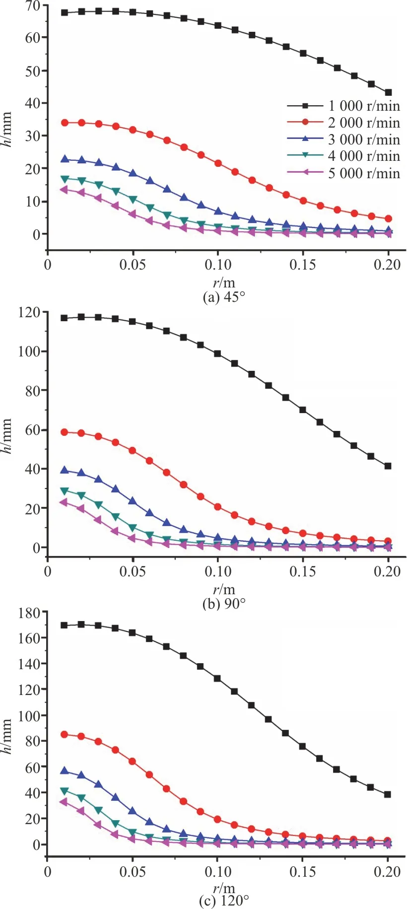
Fig.4 (Color online) Variations of half-thickness of the exit edge h against the radius r at different design speeds for different wedge angles

whereTdis the resistance moment of the blades,ωis the rotational speed, andis the amount of the vapor extracted from the supercavities (i.e., the mass flow rate of the vapor through the extraction holes located at the roots of the blades).Therefore,Tdandshould be determined to calculateEc.On one hand,Tdcan be calculated by the integral of the resistance moment imposed on the infinitesimal segment from the blade root to the blade tip.Herein,the resistance moment imposed on the infinitesimal segment can be obtained by the product of the dragFdand the radiusrcof the infinitesimal segment,whereasFdis obtained based on the results of the two-dimensional numerical simulation.On the other hand,cannot be obtained by the twodimensional numerical simulation.However, the mass of the vapor generated inside the supercavities in unit timehas the same dimension as that of.Moreover, the vapor extracted through the extraction holes comes from the generation of the vapor inside the supercavities.Hence,can characterize the desalination performance of the RSCE from another perspective.In summary, throughFdandobtained by the previous two-dimensional numerical simulations, the desalination performance of the RSCE can be estimated, which can further direct the model selection among the blade shapes with different headforms and design speeds.Thus, the time for the determinations ofTdandthrough the three-dimensional numerical simulation can be saved in the design of blade shape.Besides, the power consumed by the RSCE can be predicted by the estimatedTd, and then directing the determination of the required motor power and the selection of the motor.

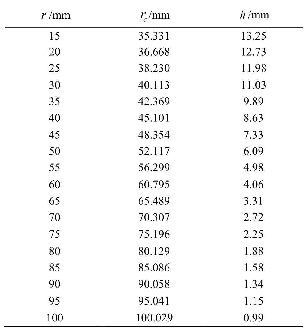
Table 1 Half-thicknesses of the exit edge (h) at different radii for the optimized blade with the wedge angle 2α=45° and design speed ωd=5000 r/min

1.2.1 Estimation of resistance moment

Through the previous two-dimensional numerical simulations[13], the relationship betweenFdand the cavitation number (or the characteristic velocityV∞)can be obtained for the cavitator with a fixedh.However, the thickness of the exit edge of a three-dimensional blade varies with the radius.Hence,the relationship betweenFdandhshould be determined in advance.To this end, we are inspired by the previous analytic study for axisymmetric cavities[15], and extend it to the cavitating flow around a planar symmetric cavitator, whose two-dimensional model is built and shown in Fig.5.The following assumptions are taken into consideration:

(1) The flow is irrotational, steady and twodimensional, while the liquid is incompressible and inviscid.

(2) The gravity and the surface tension are both neglected.

(3) The stress on the liquid-vapor interface has a unique normal component equal to the pressure inside the cavity, and is supposed to be uniform throughout the cavity.

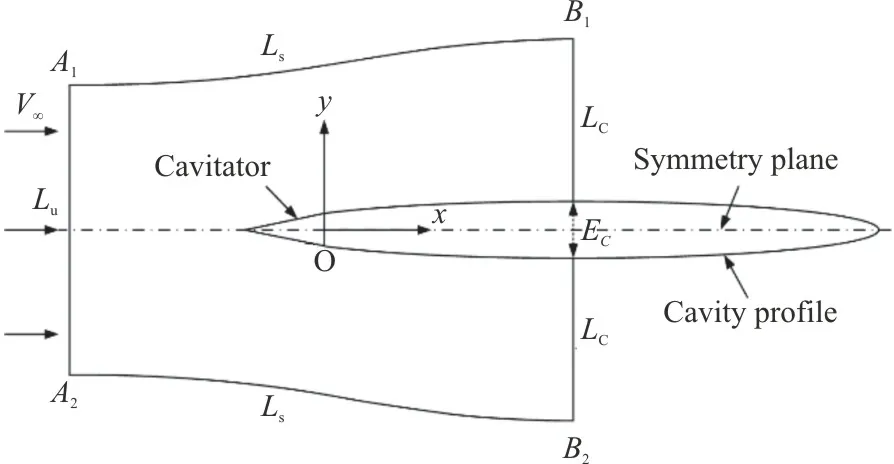
Fig.5 Two-dimensional model of cavitating flow around planar symmetric cavitator

The liquid domainA1B1B2A2with a unit length in the spanwise direction is selected as the control volume.It is limited by a lineLuat the upstream infinity, two streamlinesLsat infinity and two linesLccorresponding to an arbitrary cross section along the cavity.Besides, it is closed by the cavitator and a part of the cavity interface.According to the momentum balance of the liquid contained in the domainA1B1B2A2, we have

wherefdis the drag per unit length,pbis the pressure in the cavity,Ecis the thickness of an arbitrary cross section of the cavity,pis the pressure on the lineLc, anduis the velocity component in thex-direction.

According to the mass conservation equation

wherevis the velocity component in theydirection.

Due to the planar symmetry of the considered flow, the velocity field has no component inzdirection.Besides, the flow is assumed to be steady and the fluid is incompressible.Hence, the continuity equation is

For the cavitating flow around a slender body, the velocity componentucan be approximated by the velocity at infinityV∞, and thus the first term on the left side of Eq.(6) can be neglected.Accordingly, the velocity componentvcan be expressed as

Herein, the functionC(x) depends on the boundary condition on the cavity profiley=S(x), where the velocity is in the tangential direction to the cavity profile, i.e.,

IfLcis chosen to take its value at the location of the maximum cavity thickness, it follows that: (1)Ecis exactly the cavity thicknessEas defined in the previous two-dimensional numerical simulation[13], (2)the velocity componentvis equal to zero on the cavity profile, (3) the velocity componentvis equal to zero overLc, as indicated by Eq.(9), so that the third term on the right side of Eq.(5) can be neglected,(4) comparing with the first term on the right side of Eq.(5), the second term can be omitted due to the approximation of the velocity componentubyV∞.Ultimately, the resistance of the cavitator of a unit length in the spanwise direction is given by

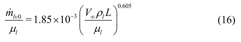
According to the empirical formulae for the cavity thickness obtained by the previous twodimensional numerical simulations[13],Eis proportional tohfor a given cavitation number.On the other hand,pbis equal topvfor the natural cavitation, so that it can be inferred from Eq.(10) thatfdis proportional toEunder a given ambient condition.Therefore,fdis proportional toh.

In order to verify the usefulness of Eq.(10), the resistance moments of the optimized blades with 2α=45° andωd=5000 r/min at different rotational speeds are estimated and compared with the results of the three-dimensional numerical simulations.The detailed three-dimensional numerical simulation will be discussed in Section 3.The dimensionless resistances per unit length (fd0ρlL/μl2, whereLis the supercavity length) of the cavitator with the base of the half-heighth0=5 mm at different dimensionless velocities (V∞ρlL/μl), are obtained based on the previous two-dimensional numerical simulation,and fitted into an empirical formula in Fig.6 as

Fig.6 Calculated and fitted dimensionless resistances per unit length fd 0ρ lL/μl2 of the cavitator with the base of half-height h0=5 mm at different dimensionless velocities V∞ρlL/μl

Therefore, the resistances per unit length is given by

Figure 7 shows the dimensionless halfthicknesses of the exit edgeh/dat different dimensionless radiirc/d, with the corresponding fitting results.The resultant empirical formula is

Ultimately, the resistance moment of the blades can be calculated by

wherer0andrtare the radii of the shaft and blade tip and equal to 0.035 m and 0.100 m for the optimized blade, respectively.By substituting Eqs.(11)-(13) andV∞=2 πωrc/60 into Eq.(14), the resistance moments imposed on the blades at different rotational speeds can be estimated, and are plotted in Fig.8, where are also shown the results obtained by the threedimensional numerical simulations for comparison.The maximum relative error of 17.8% indicates that the precision of the estimation is acceptable in engineering applications.Besides, the resistance moment is overestimated at higher rotational speeds,due to the larger supercavity size obtained by the two-dimensional numerical simulation (the comparison with the three-dimensional numerical simulation will be given in Section 3), which would cause a larger drag according to the proportional relationship between the resistance and the supercavity size.On the other hand, the resistance moment is underestimated at lower rotational speeds, due to the fact that there is no formation of cavitation behind the blades at smaller radii at lower rotational speeds (detailed results will be shown in Section 3).

1.2.2 Estimation of vapor production

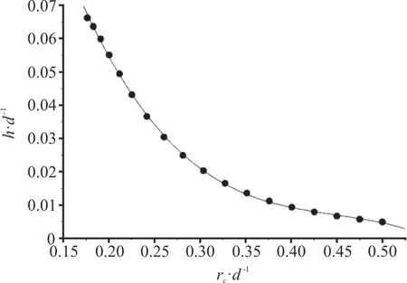
Fig.7 Dimensionless half-thicknesses of the exit ed ge h/ d at different dimensionless radii rc/ d and the corresponding fitted results

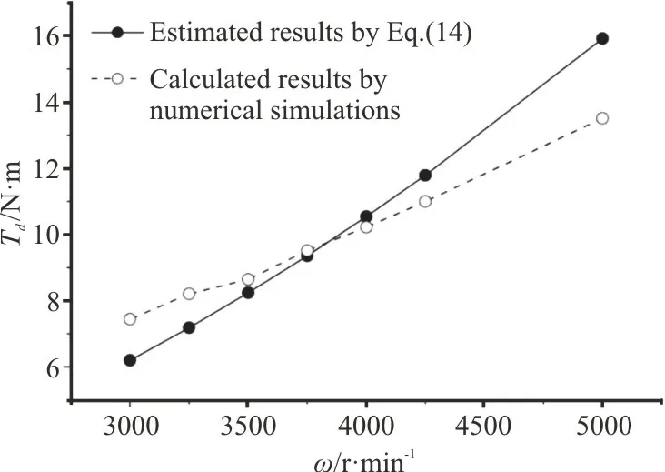
Fig.8 Estimated and calculated resistance moments of the optimized blades at different rotational speeds

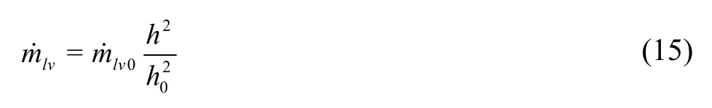
Similar to the estimation for the resistance moment, the calculatedby the two-dimensional numerical simulation is obtained for the cavitator with the base ofh0=5 mm.Thus, the relationship betweenhand the mass of the vapor generated inside the supercavity with a unit length in the spanwise direction in unit timeshould be determined beforehand.is obtained by the surface integral of the production rate of vapor (Rein Eq.(23)) within the cavity, and can be considered proportional toh2,i.e.,

where0is the mass of the vapor generated inside the supercavity with a unit length in the spanwise direction in unit time for the cavitator withh0=5 mm.The values of its dimensionless formlv0/μlfor differentV∞/(μl/ρlL)obtained by the previous two-dimensional numerical simulations are shown in Fig.9 and fitted into a formula as

The mass of the vapor generated in the supercavities behind the optimized blades in unit time can be calculated by

Ultimately,can be estimated by substituting Eqs.(13), (15) and (16), andV∞=2 πωrc/60 into Eq.(17).The estimated values at different rotational speeds are plotted in Fig.10, as well as the calculated results by the three-dimensional numerical simulations for comparison.It can be shown that the estimation method can be used to predictwith good accuracy.

Fig.9Calculated and fitted dimensionless mass of the vapor generated inside the supercavity with a unit length in the spanwise direction in unit time lv 0/μl for the cavitator with the base of half-height h0=5 mm at different dimensionless velocities V∞ρlL/μl

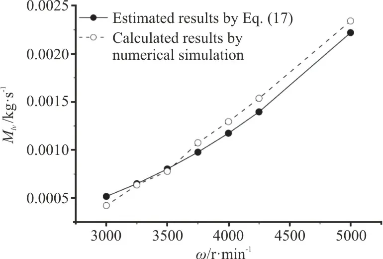
Fig.10 Estimated and calculated mass of the vapor generated inside the supercavities in unit time at different rotational speeds

According to the estimatedTdandand their comparisons with the results of the threedimensional numerical simulations, good agreements are shown, which indicates that the empirical formulae for the supercavity length obtained by the two-dimensional numerical simulations can be used for the design of RSCE’s three-dimensional blade shape.

2.Numerical method for natural supercavitating flow in RSCE

2.1 Numerical method

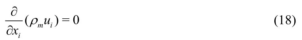
According to the previous experiments for the original cavitator[3,5], the supercavities of nearly constant sizes can be continuously generated behind the blades.Hence, the three-dimensional steady isothermal natural supercavitating flow is assumed in the present numerical simulation, which is described by multiphase flow and turbulence models.The mixture model based on the homogeneous equilibrium multiphase flow theory is selected as the multiphase flow model, in which the mixture of the gas and liquid phases is considered as a homogeneous single-phase fluid, i.e.the mixture phase[13].Accordingly, the liquid and vapor phases in this flow are modeled by solving the continuity and momentum equations for the mixture phase, and the volume fraction equation for the secondary phase, which corresponds to the vapor phase in the current simulation.

Continuity equation of the mixture phase

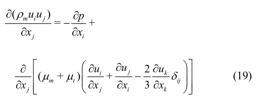
Momentum equation of the mixture phase

Volume fraction equation for the vapor phase

whereuioruj(i=1, 2 and 3,j=j=1, 2 and 3)is the velocity of the mixture phase,pis the pressure,μtis the turbulent viscosity,αvis the volume fraction of the vapor phase,ρandμare,respectively, the density and the viscosity, the subscriptsm,landvrepresent the mixture, the liquid and vapor phases, respectively.The thermodynamic properties of the liquid water and the vapor are set according to IAPWS database[14,16-17]at 25°C:ρl=997 kg/m3,μl=8.9011× 10-4Pa· s ,ρv=0.023075 kg/m3,μv=9.8669× 10-6Pa· s.The density and the viscosity of the mixture phase are defined as

ReandRcin Eq.(20) are the production rate and the condensation rate of the vapor phase, respectively,which are described by the Schnerr-Sauer cavitation model[18].

wherepbis equal topvfor the natural supercavitation, which is equal to 3169.9 Pa at 25°C as mentioned above, andRBis the radius of the bubble and defined as

wherenis the bubble number density and set to be 1×1013m-3.

wherekis the turbulent kinetic energy,εis the dissipation rate of the turbulent kinetic energy,is the velocity variance scale for the turbulent transport and can be regarded as the turbulent intensity normal to the streamlines,fis the elliptic relaxation function extracted from the source termkfin thetransport equation, andkfrepresents the redistribution of the turbulent energy from the streamwise component, the turbulent viscosityμtis defined as follows

LtandTtare the turbulent length scale and time scale, respectively, and their definitions are

The model constants in the turbulent model equations take the following values:α=0.6,C1=1.4,C2=0.3,Cε2=1.9,Cη=70,Cμ=0.22,CL=0.23,σk=1.0,σε=1.3.

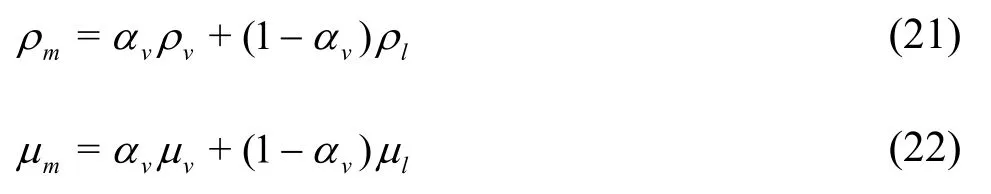
A cylinder with the heightH=100 mm and the diameterD=430 mmis selected as the computational domain, as shown in Fig.11.The height of the shaftHsis equal to 70 mm.Figure 11 also depicts the setting of the coordinate system in the simulations, in which the origin is located at the center of the computational domain.They-axis is along the blade’s entrance edge, while the rotational direction is along the positive direction of they-axis.The blades are symmetrical about the plane ofz=0 m.Both the top and the bottom of the computational domain are set to be the pressure outlet with the pressure of 101 325 Pa.The cylindrical surface is set as fixed no-slip wall, and other boundaries are set to be no-slip wall with an identical rotational speedω.The computational domain is meshed by unstructured grids with denser prismatic meshes in the boundary layer around the blades and tetrahedral meshes in the rest space.The detailed grid distribution is shown in Fig.12.In order to capture the cavity profile accurately, compared with the grids at the periphery, the grids are denser within the region where the cavities are formed.

Fig.11 Schematic diagram of the computational domain

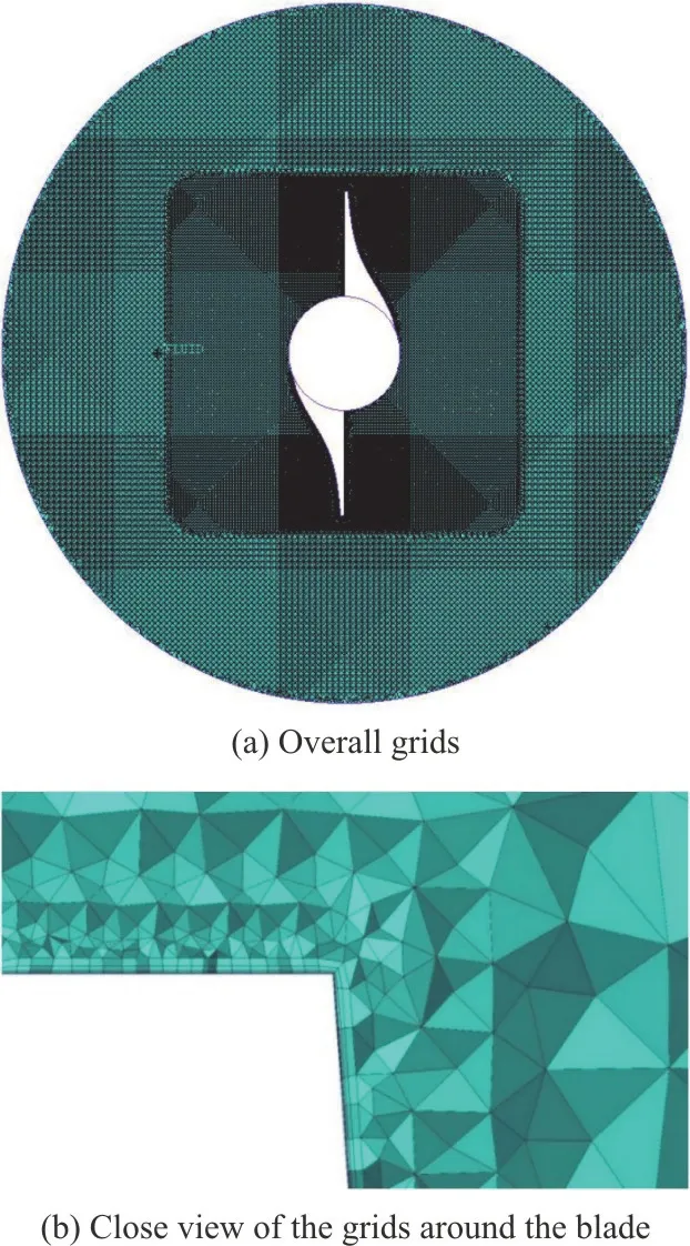
Fig.12 (Color online) Schematic diagram of the mesh generation in the computational domain

The algorithm in ANSYS FLUENT software is based on the finite volume method, and double precision is employed in the current calculations.semi-implicit method for pressure linked equationconsistent (SIMPLEC) scheme is adopted to solve the coupling of the velocity and the pressure.The pressure staggering option (PRESTO!) scheme, which is more suitable for the calculation of the cavitating flow, is adopted to discretize the pressure equation.Second order upwind scheme is used to discretize the convection terms, while the central difference scheme is used for the diffusion terms.

2.2 Mesh independence verification

The mesh independence is firstly verified for the accuracy and the economy of the calculations.Different mesh systems with gradually increasing numbers of grids are adopted to simulate the rotational supercavitating flow under the design speedωd=5000 r/min.Figure 13 depicts the variations of the surface areaAcand the volumeVcof the supercavities andTdagainst the number of grids.Herein, the profile of the cavity, based on whichAcandVcare calculated, is defined as the isosurface withαv=0.1 in this paper, as did in our previous work[13].It can be shown that the variations ofAc,VcandTdare all reduced with the increasing number of the grids, and all of them vary only slightly when the number of grids is more than 1.1×107.Therefore, the mesh system with 11 085 040 grids is chosen for the following numerical simulations.

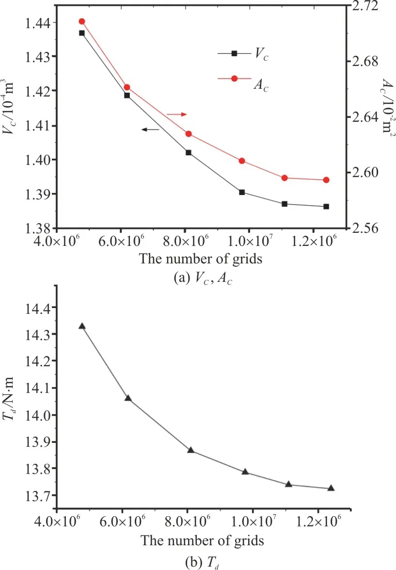
Fig.13 (Color online) Verification of mesh independence

Figure 14 shows the distribution of the dimensionless normal distance of the first grid from the wally+(y+=yuτ/ν, whereyis the wall-normal distance from the wall,,withτwbeing the wall shear stress andρbeing the fluid density andνis the kinematic viscosity)over the cavitator at the design speedωd=5000 r/min.The region withy+＜1 covers most of the cavitator’s surface, indicating that the demand of the V2F model fory+is adequately met.Moreover,ωd=5000 r/min is the highest rotational speed considered in this paper, under which the supercavities generated behind the blades occupy most of the space between the blades.A higher rotational speed would induce the closure of the cavity on the blade’s surface.Therefore, the size of the first layer of the grid adjacent the wall also satisfies the demand of the V2F model fory+at other lower rotational speeds.It is worth noting that the decrease of the local density in the cavitation region caused by the occurrence of vapor would decreasey+, which was reported to negatively affect both the accuracy and the numerical stability[20-21].Thus, a proper near-wall grid resolution should be adopted in such calculations.However, the results are found not sensitive toy+in the cavitation region in the current three-dimensional numerical simulations.

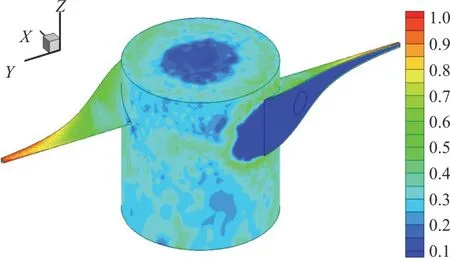
Fig.14 (Color online) Distribution of y+ over the rotational cavitator at the design speed ωd=5000 r/min

3.Results and discussions

3.1 Validation of numerical method

The numerical method developed in this paper by adopting the V2F turbulence model was validated by the simulation of the two-dimensional natural cavitating flow in our previous work[13].In order to further validate the method by the simulation of the three-dimensional cavitating flow, the model of the original cavitator designed by Likhachev[5]is used,and the numerical simulation of the rotational supercavitating flow around the original cavitator at the rotational speed of 4 690 r/min is carried out for the comparison with the experimental results[3,5].The comparison between the cavity profiles obtained by the three-dimensional numerical simulation and the experiment is shown in Fig.15.Note that the calculated cavity profile is the one within the plane ofz=0 m and depicted in red line, while the cavity profile obtained by the experiment, captured by a high-speed camera, can be considered its projection onto the plane perpendicular to thez-axis.Even so,Figure 15 reveals a good match between the results of the numerical simulation and the experiment, to validate the developed numerical method for simulating the three-dimensional cavitating flow.

3.2 Morphological characteristic

3.2.1 Supercavity shape

Fig.15 (Color online) Calculated profile of the cavity formed by the original cavitator at the rotational speed of 4 690 r/min and its comparison with experimental results[3, 5]

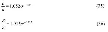
Numerical simulations are conducted for the supercavitating flows around the cavitator with the optimized blade shape at the rotational speedωranging from 3 000 r/min to 5 000 r/min.The supercavity profiles at different rotational speeds are shown in Fig.16.It can be seen that the supercavity profile is centrosymmetric about thez-axis at various rotational speeds.The supercavity enlarges with increasing the rotational speed, whose quantitative sizes (the surface area and the volume) at different rotational speeds are plotted in Fig.17.The supercavity does not completely cover the exit edge of the blade until the rotational speed exceeds 3 750 r/min.Besides, the projection of the peripheral supercavity onto the plane perpendicular to thez-axis has a shape of a smooth arc.Beyond a certain critical point downstream, the supercavity profile develops straightly toward the region of the small radius.This part corresponds to the tail of the supercavity, and its size reduces with the increase of the rotational speed.For a clearer observation, Figure 18 depicts the three-dimensional views of the supercavity profiles at different rotational speeds, which confirms the judgement for the tail of the supercavity in Fig.16.Moreover, the profile of the supercavity tail is concaved toward the inside of the supercavity, which is induced by the re-entrant jet.The flow field near the supercavity tail shown in Fig.19 indicates that the re-entrant jet at a larger velocity and in the direction towards upstream is generated right behind the supercavity, thus inducing the depression of the supercavity profile.

3.2.2 Supercavity size

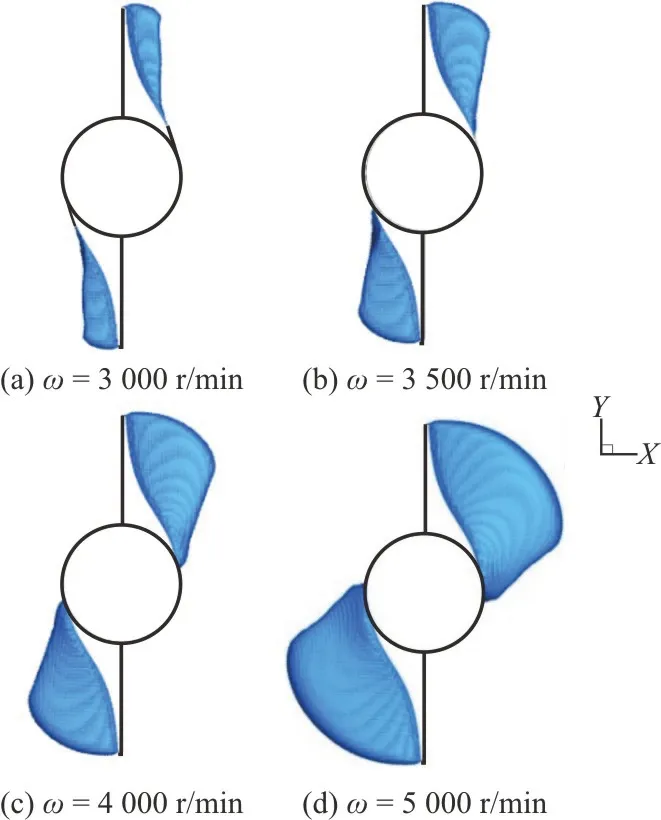
Fig.16 (Color online) Topviewsof supercavity profilesat different rotational speeds

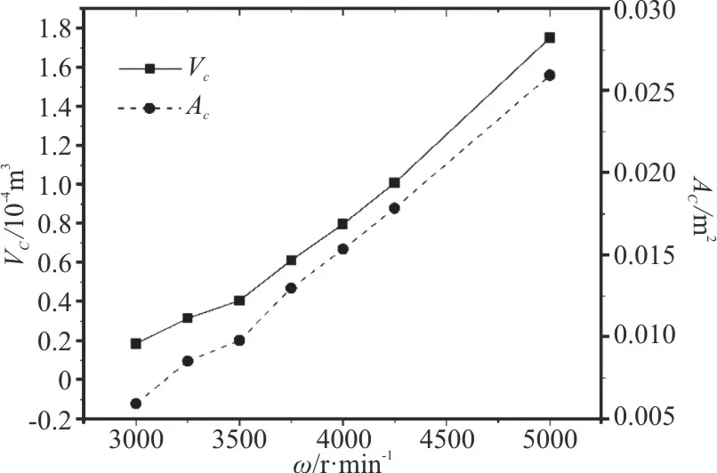
Fig.17 Volumes (V c ) and surface areas (A c ) of cavities at different rotational speeds

For a quantitative analysis, the lengths (L) and the thicknesses (E) of the supercavity at different radii at different rotational speeds are plotted in Fig.20.It is noted that the supercavity size at a certain radius is calculated by averaging the sizes of two supercavities generated behind the blades at the same radius.It is shown that both the length and the thickness of the supercavity at the same radius increase with the increase of the rotational speed.The same behavior is also observed for the variation of the supercavity length against the radius, except for the cases at larger radii.The decrease of the supercavity length with the increase of the radius at larger radii was also observed in the previous experiments for the original cavitator[3].In addition, the supercavity thickness decreases with the increase of the radius,except for those at smaller radii and at lower rotational speeds.Thus, the quantitative information about the morphology of the three-dimensional supercavity is obtained.By plotting the dimensionless supercavity lengths and thicknesses (normalized byhat the same radius) for different cavitation numbers at different rotational speeds, as shown in Fig.21, the empirical formulae for both the dimensionless supercavity length and thickness can be obtained by fitting the data as

Fig.18 (Color online) Three-dimensional cavity profiles at different rotational speeds

In the previous theoretical and experimental studies[15,22],it was concluded that the dimensionless length and thickness of the cavity are roughly proportional toσ-2andσ-1, respectively, as was also shown in our previous work based on the two-dimensional numerical simulations[13].However, Eqs.(35), (36)obtained by the three-dimensional numerical simulations in this study indicate that the exponents are deviated from the aforementioned results.To show the difference, the results of the empirical formulae obtained by the two-dimensional numerical simulations[13]are also shown in Fig.21.The difference could be attributed to the influence of the rotation, which was also mentioned in the previous design of the blade shape but without being taken into account[2].Thus it can be further found that although the estimation method based on the results of the two-dimensional numerical simulation can be used to predict the resistance momentTdand the mass of the vapor generated inside the supercavities in unit timewith an acceptable accuracy in the range of the rotational speed considered in this study, the empirical formulae obtained by two-dimensional numerical simulations cannot predict the size of the rotational natural supercavity.

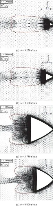
Fig.19 (Color online) Cavity profiles and velocity vectors within the cylindrical surfaces of different radii ( rc)at different rotational speeds (red line represents the cavity profile)

Fig.20 (Color online) Variations of supercavity size against the radius at different rotational speeds

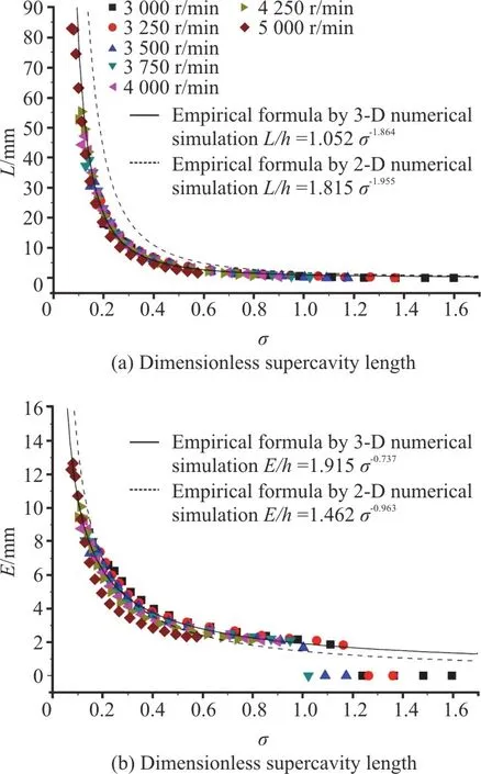
Fig.21 (Color online) Variations of dimensionless supercavity size against cavitation number at different rotational speeds

3.3 Effect of blade shape

In order to reveal the effect of the rotation alone and then to improve the empirical formulae based on the two-dimensional numerical simulations, the cavitator made up by the blades with exit edge of uniform thickness (h=5 mm) and wedge angle of 45° is considered, whose cross section is the same as the model in the two-dimensional numerical simulation, as shown in Fig.22.The cavitator has a diameter of 360 mm, and the numerical simulation is conducted at the rotational speed of 4 000 r/min.Figures 23(a), 23(b) show the variations of the supercavity length and thickness against the radius.Both the length and the thickness of the supercavity increase with the increase of the radius, except at the periphery radius position of the blade.The variation of the supercavity thickness against the radius is in an opposite trend to that for the blades with exit edge of varying thickness.The dimensionless lengths and thicknesses of the supercavity at different cavitation numbers are shown in Figs.23(c), 23(d), as well as the corresponding curve fittings.The fitted empirical formulae are as follows:

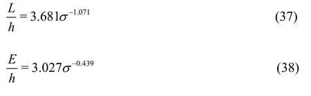
Fig.22 Cavitator made up by the blades with exit edge of uniform thickness (h=5 mm) and wedge angle of 45°

Fig.23 Variations of supercavity size against the radius and cavitation number for the blade with exit edge of varying thickness

It can be shown that the existence of the rotation would induce significant deviations of the exponents from -2 and -1, respectively.Besides, the comparisons with the dimensionless supercavity length and thickness for the blades with exit edge of varying thickness (Fig.21) also indicate noticeable differences between the empirical formulae, indicating that the dimensionless relation between the supercavity size and the cavitation number is not only affected by the rotation, but also by the blade shape.To illustrate the effect of the blade shape clearly, the dimensionless supercavity length and thickness atrc=56.299 mm(whereh=4.98 mm as shown in Table 1, to approximately represent the half-thickness of exit edge for the blades with exit edge of uniform thickness) at different rotational speeds for the blades with exit edge of varying thickness are plotted in Fig.24, as well as those with different cavitation numbers for the blades with exit edge of uniform thickness.Despite the approximation of the thickness of the exit edge, both the dimensionless length and thickness of the supercavity formed by the blades with exit edge of varying thickness are smaller than those for the blades with exit edge of uniform thickness, even at the same rotational speed of 4 000 r/min (indicated by the dashed line in Fig.24).Therefore, it can be deduced that the supercavity size at a certain location is influenced by the supercavities generated behind its adjacent blade segments.This exactly explains the formation of the cavitation atσ＞1 in this study,otherwise the cavitation cannot generally be generated at such a large cavitation number.Besides, it also illustrates that, apart from the rotation, the relationship between the dimensionless supercavity size and the cavitation number is dependent on the blade shape.

Fig.24 (Color online) Variations of dimensionless supercavity length and thickness against cavitation number for the blade with exit edge of uniform thickness (h=5 mm) and for the blade with exit edge of varying thickness at rc=56.299 mm (where h=4.98 mm )(The dimensionless supercavity length and thickness indicated by the dashed line are obtained at the rotational speed of 4 000 r/min for the blade with exit edge of varying thickness)

3.4 Discussions

It is worth noting that the supercavities do not take up most of the space between two blades at the design speedωd=5000 r/min as expected (Fig.18(g)).In fact, the empirical formula for the supercavity length obtained by the two-dimensional numerical simulation for the planar symmetric cavitating flow is directly utilized in the design of the blade shape without considering the effect of the rotation.One crucial effect is originated from the flow near the tail of the cavity, as shown in Fig.19.The local spatial circulation of the liquid resulted from the re-entrant jet would induce a highly turbulent incoming flow past the blade if its entrance edge is in the close proximity of the supercavity tail, with an irregular velocity distribution over the blade.The irregular velocity distribution would negatively affect the generation of the supercavity behind the blade.In turn, the rotation of the blade would also cause the distribution of the high pressure around the entrance edge of the blade, and then impedes the elongation of the upstream supercavity.Therefore, besides the change of the exponent in the empirical formula caused by the rotation, the interaction between the supercavity tail and the blade would also hinder the formation of the maximum possible volume of the supercavity.

Another considerable effect of the rotation is the tip and hub vortices, which would reduce the supercavity size at the root and the tip of the blade,with the deviation of the dimensionless supercavity size from the law of the exponential function, as is clearly revealed in the double logarithmic coordinate in Fig.25.Moreover, the tip vortex was observed in the previous experiments[5].Therefore, all the empirical formulae in this paper are fitted by utilizing the size of the supercavity generated by the middle part of the blade.

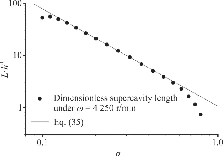
Fig.25 Dimensionless supercavity lengths for different cavitation numbers at the rotational speed of 4 250 r/min and the curve fitting based on Eq.(35)

The aforementioned effects of the rotation and the blade shape, as well as the interaction between the supercavity tail and the blade, complicate the design of the blade shape.The possible solutions are to find a more general law of how the rotation and the blade shape influence the supercavity size through studying the blade shapes with different distributions of the thickness of exit edge and different wedge angles, and to design the blade shape based on the condition ofL＜Kpwith the coefficientK＜1, as attempted by Likhachev and Li[2].

4.Conclusions

The three-dimensional blades of different sizes are designed based on the empirical formulae for the supercavity length obtained by previous twodimensional numerical simulations.The calculation method for the blade shape is also improved with better accuracy.The optimized blade shape is then determined based on the geometrical limitation and the mechanical strength.The estimation methods for the desalination performance parameters are developed to verify the feasibility of the utilization of the results obtained by two-dimensional numerical simulations in the design of the three-dimensional blade shape.Three-dimensional steady numerical simulations are conducted for the supercavitating flows around the rotational cavitator with optimized blade shape at different rotational speeds to obtain the morphological characteristics of the rotational natural supercavitation.The numerical simulation is also performed for the supercavitating flow around the rotational cavitator made up by the blades with exit edge of uniform thickness to analyze the influence of the blade shape on the morphological characteristics.The main conclusions are as follows:

(1) The blade shape with the wedge angle of 45°and the design speed of 5 000 r/min is selected as the optimized blade shape.The developed estimation methods for the desalination performance parameters can be used to predict the resistance moment and the vapor production rate inside the supercavity with acceptable accuracies, indicating the credibility of utilizing the results of the two-dimensional numerical simulations in the design of the three-dimensional blade shape.

(2) For the shape of the supercavity generated by the optimized blade at various rotational speeds, the projection of the peripheral supercavity onto the plane of the rotation has a shape of smooth arc.The tail of the supercavity behaves like a straight line towards the region of small radius in the projection onto the plane of rotation, and its profile is concaved toward the inside of the supercavity due to the re-entrant jet.

(3) Both the length and the thickness of the supercavity at the same radius increase with the increase of the rotational speed.The supercavity length increases with the increase of the radius, except for those at larger radii, while the supercavity thickness reduces with increasing radius, except for those at smaller radii and at lower rotational speeds.The empirical formulae for the supercavity size are obtained by fitting the data of the dimensionless supercavity sizes for different cavitation numbers at different rotational speeds.

(4) Comparing with the planar natural supercavitating flow, the rotation can reduce the size of the supercavity, and its detailed effects are reflected in the following three aspects: (a) The deviations of the exponents in the empirical formulae for the supercavity size from those obtained by the two-dimensional numerical simulations.(b) Hindering of the formation of the maximum possible volume of the supercavity.(c) The reduction of the supercavity size at the root and the tip of the blade and the resultant deviation of the dimensionless supercavity size from the law of the exponential function due to the tip and hub vortices.

(5) Comparing with the results obtained for the blade shape with exit edge of varying thickness, the exponents in the empirical formulae for the supercavity size for the blade shape with exit edge of uniform thickness deviate from those obtained by the previous two-dimensional numerical simulations to a relatively large extent.Besides, it can be also inferred that the supercavity size at a certain location is influenced by the supercavities generated behind its adjacent blade segments.Both facts indicate that the morphological characteristics are affected by the blade shape.

Acknowledgements

This work was supported by the International Postdoctoral Exchange Fellowship Program 2017 of the Office of China Postdoctoral Council (Grant No.20170043), the Fundamental Research Funds for the Central Universities (Grant Nos.HEUCMF180206,HIT.NSRIF.2019065), and the Basic Application Technology Research Project for the Institutes in Heilongjiang Province (Grant No.ZNGY1604).