Numerical investigation of frictional drag reduction with an air layer concept on the hull of a ship ＊

Jun Zhang, ShuoYang, Jing Liu

1. College of Aerospace Engineering, Nanjing University of Aeronautics and Astronautics, Nanjing 210016,China

2.Energy Research Institute @NTU, Nanyang Technological University, Singapore

Abstract: A novel air bubble lubrication method using the winged air induction pipe (WAIP) device is used to reduce the frictional drag of the hull of the ship and hence increase the efficiency of the propulsion system.This bubble lubrication technique utilizes the negative pressure region above the upper surface of the hydrofoil as the ship moves forward to drive air to the skin of the hull.In the present study, the reduction rate of the drag by applying the WAIP device is numerically investigated with the open source toolbox OpenFOAM.The generated air layer and the bubbles are observed.The numerical results indicate that the reduction rate of the drag closely depends on the depth of the submergence of the hydrofoil, the angle of attack of the hydrofoil, and the pressure in the air inlet.It is also proportional to the air flow rate.The underlying physics of the fluid dynamics is explored.

Key words: Winged air induction pipe (WAIP), drag reduction, frictional resistance reduction, hull of ship, OpenFOAM

Introduction

For a travelling ship, the total resistance due to the entire wetted hull consists of the viscous resistance and the wave making resistance.The coefficient of the total resistance depends on the ship speed, the hull form, the water properties and the wetted surface area of the hull.The frictional resistance is one part of the viscous resistance along with the parts due to the pressure difference, the eddies and the separation.It is caused by the viscosity of the water and the motion of the ship.As a ship speeds up or at a high Reynolds number, the flow becomes more turbulent and the thickness of the boundary layer increases.Thus the shear stress acting on the wetted surface of the hull becomes higher and the frictional resistance is increased[1].Approximately 60% of the consumed energy provided by the fuel is used to overcome the frictional resistance, a function of the viscosity of the water, the wetted surface area of the hull, and the speed of the ship[2-3].Emissions of NOxand SO2to the environment will cause air pollution[4].Therefore,various techniques were developed to reduce the frictional resistance and to increase the efficiency of the power propulsion system of the ship.One of the most popular technique is the air lubrication on the wetted hull, that is, the air is sandwiched between the water and the surface of the hull to reduce the wetted area[5].To realize it, there are mainly three kinds of methods[2]: the air film method, the cavity method,and the bubble method.The underlying physical principle and the flow features of the cavity method and the bubble method were reviewed in detail by Ceccio[6].The air film method is the most effective,but it is difficult to keep its continuity, and a huge amount of air is required.This drawback can be overcome in the cavity method by changing the shape of the hull form, but this might not be practical in some cases.On the other hand, the bubble method can retain the bubbles on the surface of the hull without modifying the hull form, and therefore it has received a wide attention from naval architects.Additionally,this method is more efficient as compared with the air film method and the cavity method.Although the air film method enjoys a higher reduction rate of the frictional resistance than the bubble lubrication method, it is difficult to form a stable air film,especially at a high ship speed[7].The efficiency of the cavity method is sensitive to the pitch and roll motions of the ship.In addition, the cavity method may cause an increase of the resistance instead in case of failing to preserve the air over the recesses[8].

Several techniques were developed to introduce bubbles to the bottom of the hull, either through the electrolysis of the water[9]or by using the compressor and porous media[10].However, these methods consume extra energy to redirect the gas to the wetted surface of the hull, thus their advantages would be lost in term of the net reduction rate of the drag.To test the efficiency of the air lubrication method on the drag reduction, experiments were conducted in a model scale by Kodama and 10%-15% drag reduction was achieved[11].Jang et al.also carried out an experiment on a model scale of the cargo vessel and estimated that the actual net reduction rate in the full scale is about 5%-6%[12].In practice, the air lubrication method was applied to an actual ship of 162m long by Mizokamietal.[13](see Fig.1(a)).Although the traditional method can achieve a reduction of 10%-15%, 5%-10% of the energy is consumed by the compressor and the porous media.The net result is only 0%-5% reduction[11].

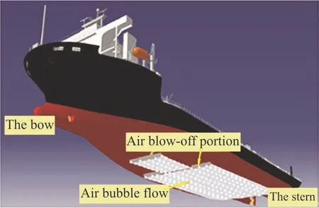
Fig.1 (a) (Color online) Bubble method applied in the sea trial[13]

Kumagai et al.[15-16]invented a novel device winged air induction pipe (WAIP) without extra energy to be consumed for the shallow draft ship.It was applied in the sea trial by Murai et al.[14]and 10% fuel can be saved (see Fig.1(b)).In this method, a hydrofoil is installed on the wetted surface of the hull as shown in Figs.2(a), 2(b).The air chamber and the pipe are integrated (Fig.2(c)).The air is driven to the wetted surface of the hull due to the negative pressure region above the upper surface of the hydrofoil where the pressure is lower than the hydrostatic pressure[16].As illustrated in Fig.2(d), an air layer and plenty of bubbles are generated in the downstream of the hydrofoil due to the Kelvin Helmholtz instability in the turbulence and the air-water interface.This phenomenon happens at the interface of multi-phase flows with different flow speeds.The generated air layer and the bubbles enter the turbulent boundary layer of the plate and the shear stress is decreased,resulting in the drag reduction.The WAIP device utilizes the kinetic energy of the moving ship to track the air, so the air compressor is not necessary for a shallow draft ship.

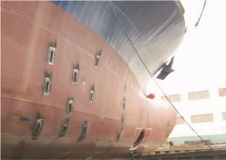
Fig.1(b) Application of winged airinduction pipe (WAIP) devices to the ship Filia Ariea[14]

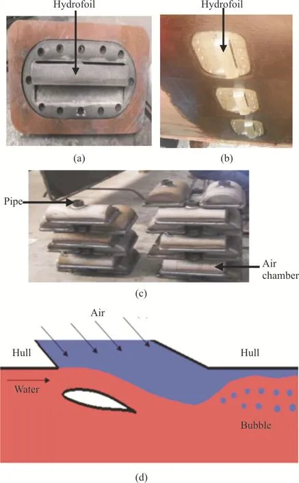
Fig.2 (Color online) Front view (a) and side view (b) of the WAIP device used on the surface of the wetted hull, (c)air chamber and pipe, and (d) cross-sectional view of the WAIP device[16]

The influence of the air injection rate and the flow speed on the drag reduction was investigated experimentally[17].It was found that at a large air flow rate and a low flow speed of the water, a great reduction can be achieved.The effect of the bubble size on the drag reduction was studied experimentally by Verschoof et al.[18]The size of the bubble was controlled by the added specific surfactants to prevent the bubble coalescence.The results show that the bubble deformability plays an important role in the drag reduction in the turbulence flow.More recently,a numerical study was carried out with commercial software Star-CCM+ to simulate the experimental testing situation[19].The same experimental conditions were applied to predict the effects of the flow speed,the orientation of the plate, and the size of microbubbles on the drag reduction.The same trend of the drag reduction was observed as in the experiment.Less efficiency was observed for the vertical plate because of the escape of the bubbles from the top.The WAIP device was applied to the actual ships in the experimental investigation by Kumagai et al.[15].The reduction rate of the drag is 10%-15%.It was found that the ship size, the number of WAIP devices, and whether a compressor is used or not, have a significant effect on the reduction rate of the drag.If the draft of the ship is shallow, the air can be driven to the wetted surface naturally and the drag reduction is achieved in a more efficient way.However, an air compressor or blower is required to retain the bubble generation under the deep draft condition (＞5 m) if the pressure over the upper surface of the hydrofoil is not low enough to overcome the high hydrostatic pressure.Furthermore,the loss control of the flow rate of the compressor can make the hydrofoil wrapped completely by the air.The formed bubbles might escape to the downstream,to affect the efficiency of the WAIP device.It is crucial to keep the air-water interface above the hydrofoil.As pointed by Kumagai et al.[15], further studies should be carried out to optimize the WAIP device and to improve the reduction rate of the drag.Given the above perspective, a numerical study is performed to investigate the effect of the hydrofoil particulars on the efficiency of the WAIP device in the present paper.

1.Numerical method

1.1 Velocity field and turbulence model

3-D, transient, viscous, incompressible, and two-phase immiscible fluid flow is numerically solved by discretizing the Reynolds averaged Navier-Stokes(RANS) equations as expressed in the tensor notations[20]:

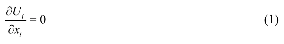
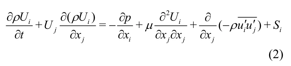
whereUiis the mean of the fluid velocity,u′is the fluctuating part, with the suffix notationsiorj=1,2,3 denoting thex-direction, they-direction,and thez-direction,ρis the fluid density,μis the fluid dynamic viscosity, pis the pressure andSiis the source term, which includes the body force and the interfacial forceFσin the present study

The closure of the turbulence model for the Reynolds stress itemis achieved by thek-ωshear stress transport (SST)[21].The turbulence kinetic energykand the specific dissipation rateωare estimated from the boundary condition of turbulence quantities, that is, the turbulence intensityIand the length scalel[22]

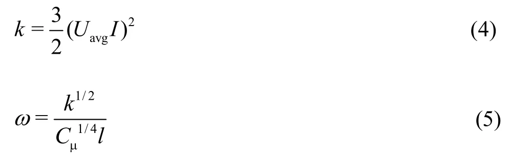
whereCμis a constant with a value of 0.09,Uavgis the averaged velocity.

Unlike thek-εandk-ωtwo-equation models, the Reynolds stress models (RSM) does not involve the isotropic viscosity assumption and can provide a superior performance for highly swirling or rotating flows and the flows with a large streamline curvature.As discussed by Khalil et al.[23], with the RSM, one can predict the separation zone more accurately based on the adverse pressure gradient.However, the RSM requires more computational time and larger CPU memory and is more difficult to converge than thek-εandk-ωtwo-equation models.In the present study, thek-ωSST turbulence model is used, with blending functions to well combine a low Reynolds numberk-ωmodel in the near-wall region and a high Reynolds numberk-εmodel in the far field.Unlike thek-εmodel,thek-ω SST model can accurately predict the boundary layer with adverse pressure gradients, for instance, in the case when the flow separation occurs on the upper surface of the hydrofoil.In addition, the large eddy simulation (LES) is costly in the computational resource requirement and is also very time consuming.Very fine grid is required near the wall to resolve the eddy viscosity.Therefore, thek-ωSST is adopted to solve the turbulent flow in the present study.

1.2 Interface solver

The air-water interface is implicitly captured by the VOF method.The advantage of the VOF method is its superior volume or mass conservation of each fluid over other methods, for example, the level-set method[24].In the VOF method, the volume fractionζis introduced and defined throughout the computational domain.The evolution of a multiphase flow system is governed by the equation

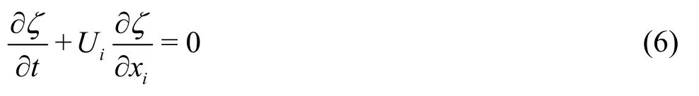
ζrepresents the discontinuous volume fraction.When the computational grid cell is fully occupied by the phase 1,ζ=1.When the computational cell is fully occupied by the phase 2,ζ=0.The interface falls in the range of 0＜ζ＜1.A typical distribution of the volume fraction is shown in Fig.3.The geometrical reconstruction method with a linearity assumption is used to reconstruct the location of the interface.Equation (6) is solved simultaneously with Eqs.(1), (2) on the same fixed grid system.Thus, the extra dynamic grid is avoided in handling the complicated interface deformation.As a result, the usage of computational memory is greatly reduced, as well as the CPU time.

For the fluid properties, the densityρand the viscosityμacross the interface are calculated with respect to the distribution of the volume fraction:

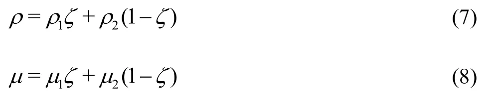
where the subscripts 1 and 2 represent the phase 1 and the phase 2, respectively.It is assumed that the fluid properties are constant within each phase.The pressure gradient across the interface contributes to the interfacial force which is the source term,governed by the momentum equation (2).The interfacial force is calculated the same as in the level-set method[24]:

σis the surface tension coefficient,κis the curvature,is the normal to the interface,φis the normal distance to the interface, andδ(x-xf)is the delta function, that is, zero everywhere except at the interface[24].It is crucial to accurately obtain the solution of the volume fractionζas it determines the value of the interface curvature, and thereby the interfacial force.The small error may accumulate to a significant error for the interface properties,consequently, to badly affect the solution of Eqs.(1),(2).The solution of the interface is quite sensitive to the grid resolution.That is, the finer the grid, the more accurate the interface solution.But the accuracy of the solution requires the CPU cost and the computational time.In the following numerical simulation, the experimental results are used to verify the grid resolution and the numerical method.

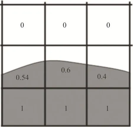
Fig.3 Volume fraction values ζ

1.3 Discretization method

The unstructured grid is created with the software ANSYS ICEM CFD to divide the computational domain into grid cells and to store the fluid properties.2-D simulation is carried out and a pseudo-3D approach is adopted with only one grid layer generated inz-direction.The governing Eqs (1), (2)and (6) are written in a form of the standard transport equation, which can be discretised with the finite volume method (FVM).The solver inter Foam built in the open-source CFD toolbox OpenFOAM is used to solve the fluid flow.The first order Euler implicit differencing scheme is used for the temporal discretization, with the time step self-adaptive based on the condition that the maximum Courant number CFL＜0.5 in order to ensure the stability and the convergence of the computing iteration.Other numerical schemes used to discretize the derivatives in the transport equation along with the interpolation method are listed in Table 1.Gauss stands for the standard Gaussian finite volume integration and followed by the interpolation scheme.The numerical schemes are described in detail in the OpenFOAM user guide and will not be repeated here.The pressure implicit with splitting of operators (PISO) method is used for the pressure-velocity coupling.

Table 1 Discretization scheme and interpolation method used in the solver

2.Numerical results and discussion

2.1 Validation of numerical method for multiphase flows

The influence of the hydrofoil on the free surface of the water is a critical hydrodynamic problem to validate the accuracy of the numerical method for multiphase flows.An experiment on the wave propagation caused by a towed hydrofoil was carried out by Duncan in an opening water tank of 24.00 m long, 0.61 m wide, and 0.61 m deep[25].The employed profile is NACA0012 with the chordc=0.203m ,the angle of attackα=5°, and submerged 0.185 m deep (0.91c).Its distance to the tank bottom is 0.175 m.The hydrofoil’s span is 0.60 m with a clearance of 2 mm to 5 mm between the hydrofoil edges and the tank side walls.2-D effect is obtained in that experiment as stated by Duncan.Therefore, a 2-D numerical simulation should be sufficient to capture the wave propagation produced by the moving hydrofoil under the similar experimental conditions.The towing speed of the hydrofoil is 0.8 m/s in the experiment whereas the hydrofoil is stationary and the water is moving in the numerical simulation according to the relative motion principle.The computational domain has 5cin the upstream and 10cin the downstream from the centre of the hydrofoil.The initial still free surface is 4caway from the upper boundary as shown in Fig.4(a).It has to be pointed out that the distance from the hydrofoil to the tank bottom is 0.175 m in the experiment, but this distance is 1.218 m (6c) in the simulation as did by Karim et al.[26]in order to secure the convergence of the simulation.As illustrated in Fig.4(a), the velocity inlet and pressure outlet boundary conditions are applied for the inlet and outlet boundaries,respectively.The symmetric condition is specified for the upper and lower boundaries.A no-slip condition is applied for the hydrofoil.The turbulence intensity is 1% and the turbulence length is 1c.The hybrid grid is generated in the computational domain, that is, the rectangle grid is created near the free surface and the rest is the triangle grid as shown in Fig.4(b).

Fig.4 (a) Computational domain, free surface, applied boundary conditions

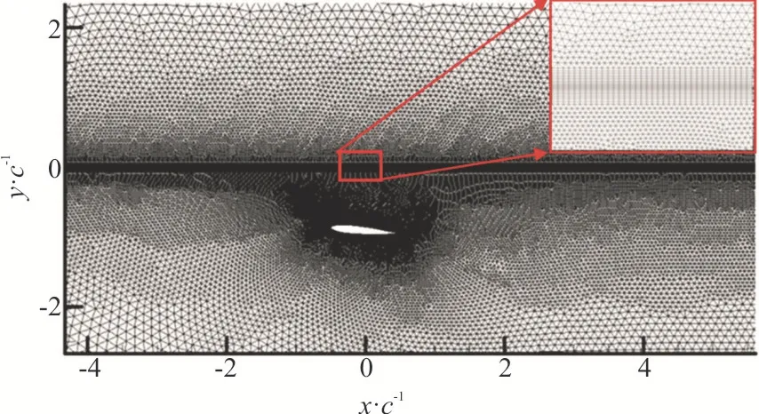
Fig.4 (b) (Color online) Zoomed-in view of the computational grid used in the numerical simulation

The grid independence study is performed first in order to obtain the grid converged solution of the free surface dynamics.Three grids are considered, with M0=105693, M1=179994 and M2=319 697.Figure 5(a) shows the hydrofoil-produced wave profile.The results of M0 and M1 are almost identical except the last wave crest.By comparing with the experimental results[25], a good agreement is achieved in term of the wave length 2c.However, the hydrofoil-produced waves are damped out faster in the experimental results than in the numerical results.This could be due to the influence of the shallow tank bottom in the test as mentioned by Duncan[25].The distance between the hydrofoil and the tank bottom is only 0.175 m.The resistance of the bottom could exhaust a part of the wave energy and leads to a strong damping.On the contrary, in the numerical calculation,the influence of the bottom is eliminated because the hydrofoil is 1.218 m far away from the lower boundary, where the symmetric condition is applied(Fig.4(a)).Thus, the free surface elevation is still relatively higher after one period.The coefficient of the liftCLof the hydrofoil versus the number of grid cells is plotted in Fig.5(b).CLis defined asCL=L/(0.5ρU2), whereLis the lift.The flow is closely related with the pressure difference, which accounts for the lift and the drag on the hydrofoil.The difference ofCLbetween the grids M0 and M1 is less than 2%.It can be concluded that the grid M0 is fine enough to carry out the numerical simulation on the free surface evolution.

Fig.5 (Color online) Numerical results with different numbers of grid cells compared to the experimental results

To further validate the accuracy of the grid M0 and the applied numerical method, an additional two different incoming flow speedsUare simulated,namely, 0.6 m/s, 1.0 m/s.The corresponding Reynolds numbersReare 1.1×105, 1.9×105.HereReis defined as

The obtained wave length is compared with the experimental results as shown in Fig.6.A good agreement is achieved, which further shows that the resolution of the grid M0 and the present numerical method are effective in capturing the evolution of the air-water interface and are sufficient to be used in the following WAIP numerical investigation of the multiphase flow system.

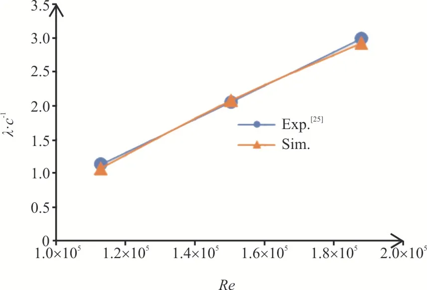
Fig.6 (Color online) Water wave length versus different incoming flow speeds

2.2 WAIP device

2.2.1Problem description and parametric study

In this section, the numerical simulation is carried out to investigate the reduction rate of the drag of the WAIP device.Although the hull of the ship is in a curved form as shown in Fig.1(b), the hull is assumed to be straight locally and is in the horizontal orientation.It is submerged 5 mm deep in the water on a model scale.NACA653618 is employed with the chordc=40 mm and the angle of attackα.Its distance to the plate ish.A schematic diagram of the WAIP device together with the 2-D computational domain is illustrated in Fig.7.A pipe of 0.20cin diameter is connected to the air chamber.The air compressor can be connected to the pipe if necessary.Between the air chamber and the opening hole is the air duct.The angle of the duct is the same as presented in the publication[16].The computational domain is 55cwide and 25chigh.The water flows from left to right beneath the plate with a speed of 1 m/s corresponding to a Reynolds numberRe=0.4× 105.The velocity inlet and pressure outlet conditions are applied for the inlet and the outlet.The right upper corner of the domain is the air outlet with a high pressure of 49.05 Pa, which is equivalent to the plate submerged 5 mm deep in the water.The unstructured triangle grid is generated throughout the computational domain and the fine grid is used around the hydrofoil as shown in Fig.8.The same numerical method is applied as stated in Section 2.

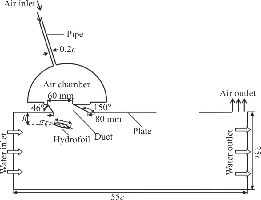
Fig.7 Schematic view of the computational domain used for the WAIP device simulation

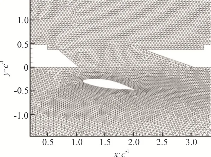
Fig.8 Zoomed-in grid around the hydrofoil

The parametric study is carried out for various values of the hydrofoil depthh(0.25c,0.375c,0.5c, 1cand 1.5c), the air pressure in the inletp0(0 Pa, 50 Pa, 100 Pa, 150 Pa), andα(8°, 12°, 16°,20° and 24°).All study cases and numerical results are listed in Table 2.The coefficient of the drag is defined asCD=F/(0.5ρU2S) , whereFis the frictional drag on the plate, the incoming flow speed of the waterU=1m/s,Sis the reference area,namely,cin the 2-D case.For the case A12 without the hydrofoil involved,CDis 0.0932, the highest one over other cases.ΔCDis the reduction rate of the drag with respect to the case A12.

In order to study the influence of the hydrofoil on the frictional drag reduction, the case A12 without the hydrofoil is studied first.The air pressurep0in the inlet is 0 Pa.The numerical results of the volume of fluid are shown in Fig.9.The red region represents the water and the blue region represents the air, and VOF=0.5 is the air-water interface.Bubbles are formed from the air-water interface due to the Kelvin-Helmholtz instability.The air flow rateQthrough the pipe is 2.09×10-4m3/s as given in Table 2.

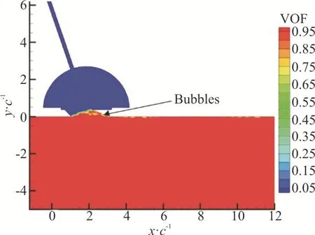
Fig.9 (Color online) Volume of fluid in case A12 without the hydrofoil

The numerical results of the volume of fluid in the case A2 are shown in Fig.10(a).The hydrofoil is submerged 0.375cdeep withα=12°.The presence of the hydrofoil changes the behaviour of theair.The air layer is formed at the bottom surface of the plate due to the negative pressure over the upper surface of the hydrofoil as shown in Fig.10(c).The pressure jump occurs across the air-water interface.The velocity of the air above the interface is much lower than that of the water below the interface (Fig.10(b)).The velocity shear contributes to the Kelvin-Helmholtz instability and leads to the bubble break-off from the end of the air layer.The formed bubbles travel along the surface of the plate and finally escape from the air outlet.The air has to continuously flow into the pipe at a rate of 5.55×10-4m3/s to supplement the escaped bubbles.With the air lubrication to the surface of the plate, a 23.2% reduction rate of the drag is achieved.Figure 10(d)shows the streamlines of the fluid flow, the vortices are formed inside the air chamber and the air layer flows out from the duct.The shear vortices are visible at the end of the air layer.

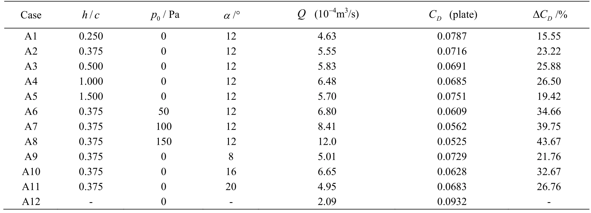
Table 2 Numerical results of the parametric study for the depth of submergence of the hydrofoil h, the air pressure p0 in the inlet, and α

2.2.2Effect of depth of submergence of the hydrofoil

A direct comparison of the interface profile is given in Fig.11.The numerical results of the volume of fluid by varying the depth of the submergence of the hydrofoilh(0.25c,0.375c, 0.5c, 1cand 1.5c) are presented in Fig.12.The applied flow condition is the same as in the case A2 in the numerical simulation.The results show that with the increase ofh, the thickness of the air layer increases whenh＜0.5cand decreases whenh≥0.5c.The influence ofhon the air blow-off can be explained with the results of the pressure distributionprghin Fig.13.As the hydrofoil moves deeper, the negative pressure region over its upper surface is enlarged,which is favourable for more air being sucked through the duct (Fig.11,h=0.25c, 0.375cand 0.5c).Then the air layer grows much thicker.However, after a certain depthh=0.5c, the negative pressure region in the downstream starts to dominate the behaviour of the air blow-off, the air layer is stretched longer instead of thicker.When the hydrofoil is too far away from the plate when the pressure above the upper surface of the hydrofoil is fully developed, the negative pressure region in the downstream is almost vanished (Fig.13(e)) and the air layer becomes the thinnest and flat as shown in Fig.12(e).The longer bubbles are formed instead of the dispersed small bubbles as shown in Figs.12(a)-12(d).

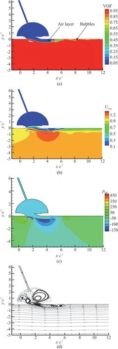
Fig.10 (Color on line) Volume of fluid ( a), velocity magnitude(m/s) (b),pressure distributionprgh (Pa) (c),and streamlines (d) the case A2 with the hydrofoil

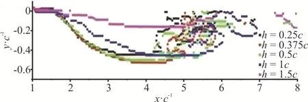
Fig.11 (Color online) Interface profiles caused by hydrofoil at different water depth h

As presented in Fig.14, the reduction rate of the drag ΔCDand the air flow rate have the same trend and both reach the maximum ath=1c.The increased air flow rate fromh=0.25ctoh=1cis to accommodate the increased air layer length.Hence,the reduction rate of the drag is increased since the larger surface area is covered within the turbulent boundary by the bubbles.The maximum ΔCDoccurs ath=1cwhen the air layer is the longest (Fig.12)and the low-pressure region in the downstream of the hydrofoil is the largest (Fig.13(d)).Both ΔCDandQstart to decrease whenh＞1c.As the hydrofoil is too far away from the plate whenh=1.5c, the low pressure region in the downstream of the hydrofoil is vanished (Fig.13(e)), then a few thinner and longer droplets are formed over the surface of the plate (Fig.12(e)).The effectively covered area by the bubbles within the turbulent boundary layer is reduced.The above results reveal that the reduction rate of the drag is dependent on the depth of submergence of the hydrofoil.

2.2.3Effect of the Pressure in the Air Inlet

Fig.12 (Color online) Results of volume of fluid by varying depth of hydrofoil

Fig.13 (Color online) Results of the pressure distribution prgh (Pa) by varying the submerged depth of the hydrofoil

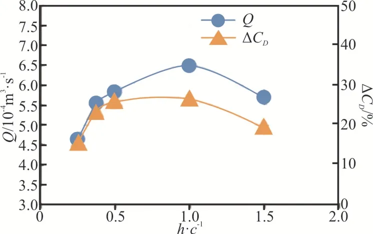
Fig.14 (Color online) Air flow rate and reduction rate of drag at different water depth of the hydrofoil

As stated by Kumagai et al.[16], under the deep draft condition of the ship, an air compressor has to be used to pump the air to the bottom of the ship’s hull to preserve the formed air layer.So the effect of the pressurep0in the air inlet on the reduction rate of the drag will be investigated.The studied pressure range is 0 Pa-150 Pa.Figure 15 shows the numerical results of the volume of fluid.Comparison of the interface profiles under different pressure conditions is presented in Fig.16.The increased pressure causes the air layer grow longer and thicker, and consequently the air flow rate increases from 5.55×10-4m3/s at 0 Pa to 1.20×10-3m3/s at 150 Pa as shown in Fig.17.Associated drag reduction is therefore enhanced accordingly since the covered area on the plate surface is enlarged.The reduction rate of the drag ΔCDreaches 43.67% at 150 Pa.It has to be pointed out that the present ΔCDdoes not take account of the consumed energy provided by the compressor.

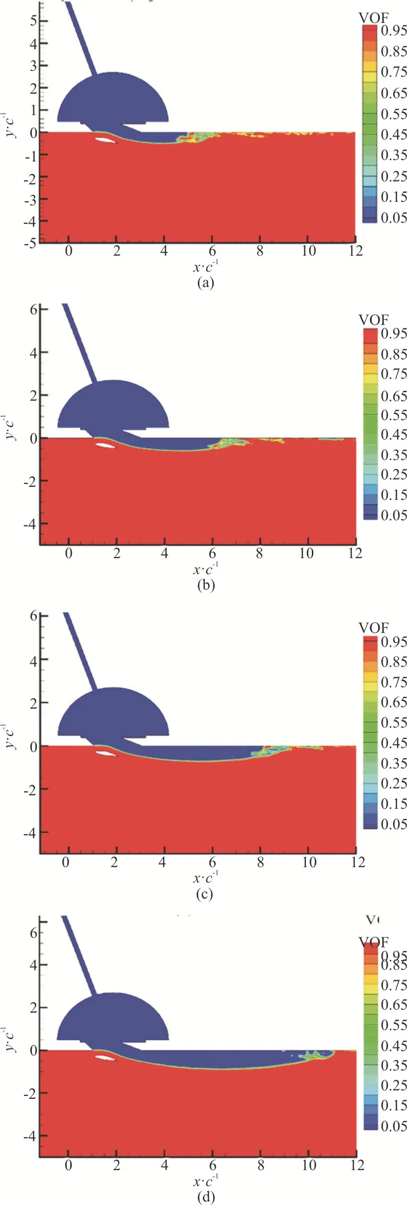
Fig.15 (Color online) Volume of fluid with different pressure p0 at the opening hole

2.2.4Effect of angle of attack()α

Fig.16 (Color online) Interface profiles caused by the hydrofoil at different pressure p0 in the air inlet

Fig.17 (Color online) Air flow rate and reduction rate of drag versus the pressure p0 in the air inlet

The effect ofαon the reduction rate of the drag of the WAIP device is studied in this section including the cases A2 and A9-A11 (Table 2).The results of the volume of fluid are shown in Fig.18.The higher angle of attack can deflect the flow downward and thereby the air layer becomes thicker.But whenα=20°, the air layer becomes susceptible to break because the Kelvin-Helmholtz instability becomes imminent.As a result, the bubbles are likely break-off due to the unstable interface and the higher discontinuity of the velocity between two phases.In fact, this is unfavourable for the drag reduction.Direct comparison of the interface profiles at different angles of attack is shown in Fig.19.The interface profile above the hydrofoil traces the outline of the hydrofoil,and the thickness of the air layer increases with the increase ofα.To clearly demonstrate the fluid behaviour, the streamlines are plotted in Fig.20.The shear flow-induced vortices are observed inside the air layer and the bubbles.Figure 21 shows the pressure distribution of the fluid field at different angles of attack.The flow separation happens at the vicinity of the trailing edge of the hydrofoil and leads to an enlarged low pressure region formed in the downstream.So more air is sucked in and consequently the air flow rate increases.Figure 22 shows the trends of the reduction rate of the drag and the air flow rate, and both are consistent with the highest values atα=16°.The decrease of the reduction rate of the drag atα=20° is due to the early bubble break-off as shown in Fig.19.It is visible that the stagnation at the leading edge of the hydrofoil is stronger asαincreases (Fig.21), which indicates that the hydrofoil must resist a higher drag from the flow.

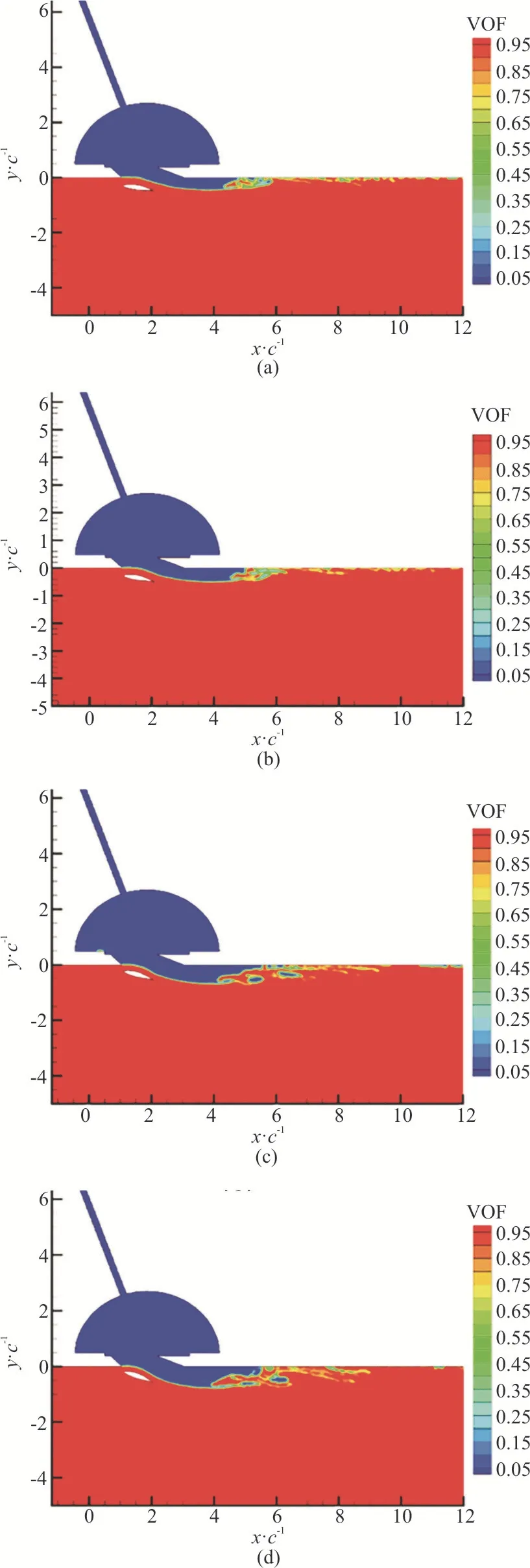
Fig.18 (Color online) Volume of fluid with different angles of attack

Fig.19 (Color online) Interface profiles caused by the hydrofoil at different angles of attack

3.Conclusion

The parametric study is carried out numerically for the drag reduction of the WAIP device for its possible use on the hull of the ship.The open source CFD toolbox OpenFOAM is employed.The RANS equations and the VOF method are used to solve the multi-phase flow and precisely capture the air-water interface.The results are validated with the published experimental results.A good agreement shows the reliability of the present numerical method for the calculation of the air-water interface evolution.The parametric study is carried out to investigate the WAIP device with respect to the effects of the depth of submergence of the hydrofoil, the pressure in the air inlet, andαon the reduction rate of the drag.The underlying physics is analyzed and explored numerically.Overally, it is found that the reduction rate of the drag has a similar trend as the air flow rate.The numerical results reveal that the reduction rate of the drag closely depends on the depth of the submergence of the hydrofoil andα.The underlying scientific principle is explored based on the fluid dynamics.The Kelvin-Helmholtz instability and the bubble break-off are observed.The effect of the pressure in the air inlet is also examined.However,the consumption of energy to run the air compressor is excluded in the present study.The benefit of the compressor application requires the sea trial to show its efficiency on the drag reduction.In addition, it has to be pointed out that the frictional drag on the plate is only considered and the drag caused by the hydrofoil is not included.On this point, the study of the optimization of the NACA series of the hydrofoil should be carried out in future to minimize the drag caused by the hydrofoil.On the other hand, the accuracy of the used turbulence model should be validated with experimental data.So it is worth to apply different turbulence models to predict the multiphase flow physics for the instability of the interface in future work.Although it could be more accurate to model the flow structure with the 3-D study, the computational resource and time will be much costly to capture the droplet break off and theevolution of all droplets because of the used large number of mesh cells.Some generated mesh cells have to be smaller than many formed tiny droplets.The intention of the 2-D study in this present paper is to narrow down the parametric study ranges according to the obtained qualitative trend of the drag reduction.In future, the selected effective methods can be investigated in the 3-D simulation, for example,

h/c=0.25, 0.50,α=12°, 16°.

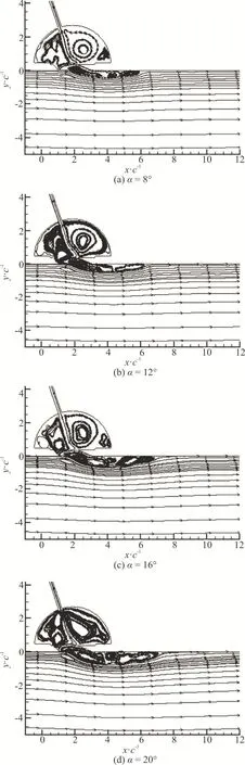
Fig.20 Streamlines of the flow field at different angles of attack

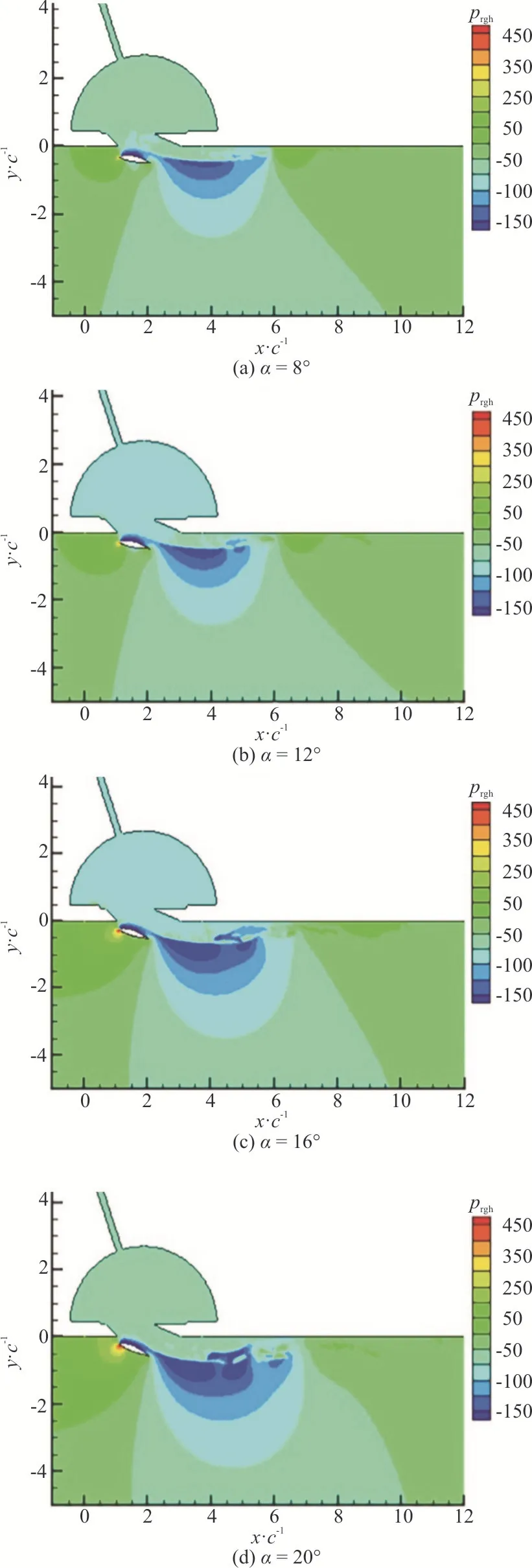
Fig.21 (Color online) Pressure distribution (Pa) of the flow field at different angles of attack

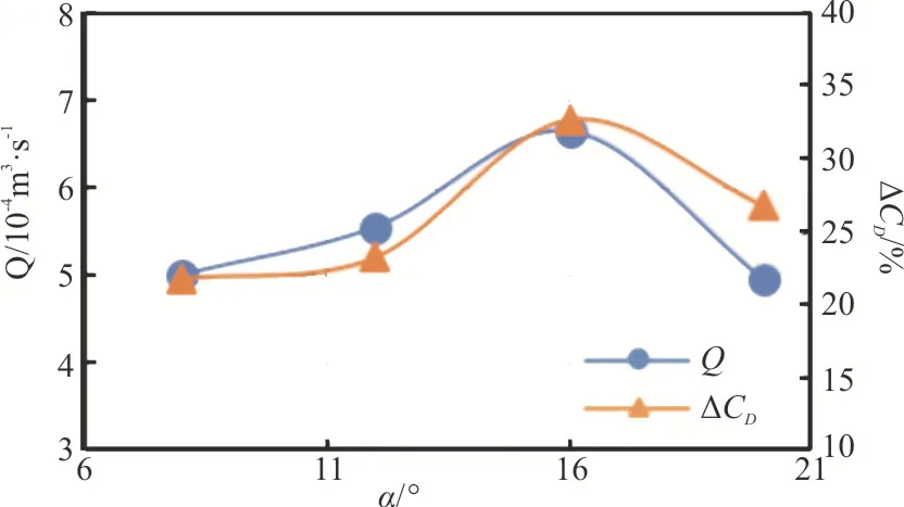
Fig.22 (Color online) Air flow rate and reduction rate of drag of the numerical results at different angles of attack

Acknowledgements

This work was supported by the Key Laboratory fund for Hydrodynamics (Grant No.6142203180304).