Can Langmuir Circulations Solve the Problem of Insufficient Upper-Ocean Mixing?

HUANG Chuanjiang, QIAO Fangli, 3), and DAI Dejun, *

Can Langmuir Circulations Solve the Problem of Insufficient Upper-Ocean Mixing?

HUANG Chuanjiang1), 2), QIAO Fangli1), 2), 3), and DAI Dejun1), 2), *

1) First Institute of Oceanography, Ministry of Natural Resources, Qingdao 266061, China 2) Laboratory for Regional Oceanography and Numerical Modeling, Pilot National Laboratory for Marine Science and Technology, Qingdao 266237, China 3) Key Laboratory of Marine Sciences and Numerical Modeling, Ministry of Natural Resources, Qingdao 266061, China

Insufficient vertical mixing in the upper ocean during summer is a common problem of oceanic circulation and climate models. The turbulence associated with non-breaking waves is widely believed to effectively solve this problem. In many studies, non-breaking surface wave processes are attributed to the effects of Langmuir circulations (LCs). In the present work, the influences of LCs on the upper-ocean thermal structure are examined by using one-and three-dimensional ocean circulation, as well as climate, models. The results indicated that the effect of vertical mixing enhanced by LCs is limited to the upper ocean. The models evaluated, including those considering LC effects alone and the combined effects of LCs and wave breaking, failed to produce a reasonable summertime thermocline, resulting in a large cold bias in the subsurface layer. Therefore, while they can slightly reduce the biases of mixed layer depths and sea surface temperatures in models, LCs are insufficient to solve the problem of insufficient vertical mixing. Moreover, restriction of non-breaking surface wave-induced processes in LCs may be questionable.

Langmuir circulations; vertical mixing; thermocline; subsurface temperature; non-breaking wave processes

1 Introduction

Vertical mixing plays a key role in regulating the temperature structure and circulation of oceans. Insufficient mixing in the upper ocean during summer is a common problem of oceanic circulation and climate models that usually results in extremely high sea surface temperatures (SSTs) and extremely low subsurface temperatures (Martin, 1985; Ezer, 2000; Huang, 2011). Huang, (2014) assessed the ability of 45 Coupled Model Inter-comparison Project Phase 5 (CMIP5; Taylor, 2012) models to simulate the surface mixed layer and found that the summer mixed layer depth (MLD) is significantly underestimated in most of these models. The authors thus suggested that this systematic underestimation of MLD is caused by insufficient upper-ocean vertical mixing in the climate models.

Surface gravity waves can greatly enhance the turbulence kinetic energy (TKE) and associated vertical mixing of the upper ocean through wave-breaking and non-breaking processes (Agrawal, 1992; Drennan, 1996; Young and Babanin, 2006) and effectively correct the problem of insufficient mixing (Huang, 2011; Qiao and Huang, 2012). Most of the wave energy is dissipated locally through wave breaking (Donelan, 1998). However, vertical mixing associated with wave breaking alone is insufficient to significantly improve simulations of the upper ocean (Zhang, 2007; Huang, 2011) because such mixing is mainly confined to the near-surface zone with a depth scale of the wave height (Rapp and Melville, 1990; Craig and Banner, 1994; Soloview and Lukas, 2003).

Recent research efforts have focused on the effects of non-breaking waves. Because surface waves are inherently nonlinear in real oceans, they are not truly potential waves prior to breaking (Phillips, 1961). Non-breaking surface waves can directly regulate turbulence and mixing in the upper ocean. Compared with breaking waves, non-breaking waves can influence larger depths and are moresignificant for upper-ocean mixing (Anis and Moum, 1995; Gemmrich and Farmer, 2004).

Langmuir circulations (LCs), which are associated with the Stokes drift induced by surface waves, are among the most obvious phenomena in the surface layer; they usually occur as organized large-scale convective motions in the sea surface. When LCs appear, they rapidly mix away near-surface stratifications, decrease the SST, and deepen the mixed layer (Weller and Price, 1988). Therefore, LCs are extensively used to improve simulations of the upper ocean, especially the MLD (Li, 1995; Li and Garrett, 1997; Kukulka, 2009; Belcher, 2012; Li, 2016; Ali, 2019). The available studies originated from large-eddy simulations (LESs) (Skyllingstad and Denbo, 1995; McWilliams, 1997; Noh, 2004) and were subsequently extended to oceanic circulation (D’Alessio, 1998;Kantha and Clayson, 2004) and climate (Dufresne, 2013; Fan and Griffies, 2014) models; here, non-breaking wave-induced mixing was attributed to effects of LCs (Leibovich and Paolucci, 1980; McWilliams, 1997; Grant and Belcher, 2009).

In the present paper, we assessed the role of LCs in upper-ocean mixing by examining their influences on upper-ocean thermal structures and then determined whether attributing non-breaking wave-induced mixing to the LCs is reasonable. In Section 2, we briefly review two parameterizations of the LCs used in subsequent sections. We then examined the effects of LCs on regulating the temperature profiles of the upper ocean by using a one-dimensional model in Section 3 and a three-dimensional model in Section 4. Four CMIP5 models consider the effects of LCs (Huang, 2014); in Section 5, the abilities of these models to simulate subsurface temperatures are analyzed. Section 6 provides the conclusions of this study.

2 Parameterization of LCs

The effects of LCs have been incorporated into various vertical mixing schemes, such as the Price-Weller-Pinkel model (Li, 1995; Li and Garrett, 1997), the turbulence closure model (D’Alessio, 1998; Axell, 2002; Kantha and Clayson, 2004), and the K-profile parameterization model (McWilliams and Sullivan, 2000; Smyth, 2002). Most classical turbulence closure models add an additional turbulence production term associated with the Stokes drift. Kantha and Clayson (2004) incorporated the effects of LCs into the Mellor-Yamada (M-Y) turbulence model (Mellor and Yamada, 1982), in which the two prognostic equations for2and2are as follows:

The turbulence production associated with the Stokes drift can be written as

whereuandvare the Stokes drift velocities andandare the fluctuations of horizontal velocity components.

In this scheme, a new constant6is introduced. Harcourt (2013) showed that selecting a value for6presents a tuning dilemma between minimizing errors in predicting the mixing length and minimizing errors in predicting TKE.6is expected to be of the order of magnitude of1(Soloviev and Kukas, 2006). However, increases in the vertical mixing coefficient strongly depend on this constant in this scheme (Kantha and Clayson, 2004); thus, it is usually set to 7.2 (Kantha, 2010), which is much larger than1(usually set to 1.8), to fit the LES results of Mc- Williams(1997).

Axell (2002) introduced the effects of LCs into a-turbulence closure model in which the turbulence behavior induced by LCs is similar to those induced by the mean current shear and internal waves. The total shear production is

wherePis the turbulence production induced by breaking internal waves andPis the shear production by LCs, which is given by

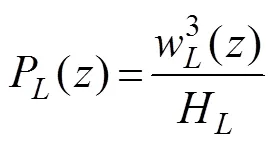
in which() is the local buoyancy frequency. Moreover,

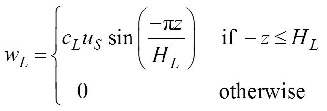
is the velocity scale associated with the LCs andcis a non-dimensional constant usually set to 0.15.

3 One-Dimensional Experiments

3.1 Model Description

In this section, a one-dimensional model is used to examine the behavior of LCs compared with field observations from June 2007 to January 2008 taken from Ocean Weather Station Papa, which is located in the eastern North Pacific at 145˚W, 50˚N. This model is similar to that used by Mellor and Blumberg (2004). The water depth is set to 200m with a model vertical resolution of 2m. The initial temperature and salinity are taken from values recorded on June 9, 2007 and linearly interpolated to the model grid; the initial velocity is set to zero. Hourly surface data are used to force the numerical model. Because a net surface heat imbalance was previously found at this site (Large, 1994), 15Wm−2is added to the outgoing heat flux to decrease the simulated deviation. In addition, the SST and sea surface salinity (SSS) are relaxed to the field observations, with relaxations of 50Wm−2K−1for SST and 30 days for SSS (assuming a MLD of 25m). Other details are provided in Huang(2011).

Three cases, named experimentP, experimentP, and experimentP, were carried out to evaluate the effects of LCs on the upper ocean (Table 1). The first case is based on the original M-Y scheme, in which the effects of surface waves are not included. In the second case, the scheme of Kantha and Clayson (2004) is used to describe LC effects. Some studies have suggested that the combined effects of LCs and wave breaking can produce strong vertical mixing in the upper ocean (Sullivan, 2007). Therefore, wave-breaking effects are considered in the third case, in which the scheme of Mellor and Blumberg (2004) is used.

Table 1 Experiments conducted by using one-dimensional and three-dimensional models

Notes: Each group of experiments includes three cases: 1) A control experiment, in which the effects of surface waves are not included; 2) a test case that includes LC effects as in Eqs. (1) and (2); and 3) a test case that includes the combined effects of LCs and wave breaking.

3.2 Results

The most notable features induced by insufficient upper-ocean vertical mixing are a too-sharp model summertime thermocline and its associated too-cold subsurface temperature (Ezer, 2000; Huang, 2011). Fig.1 shows simulated and observed daily-mean upper-ocean temperature profiles. As expected, the summertime thermocline in experimentPis shallower and sharper in comparison with field observations due to insufficient vertical mixing. This unrealistic thermocline results in an overly low simulated subsurface temperature in summer. The maximum bias of the subsurface temperature can reach up to −4℃ in experimentP(Fig.2a).

The cold bias is somewhat reduced when LC effects are included. However, this improvement is mainly limited to the base of the mixed layer, and its maximum value is only 2℃ (Fig.2b). The combination of LCs and wave breaking enhances their individual roles and transfers more energy into deep layers (Sullivan, 2007; Li, 2013). When LCs work together with wave breaking, the simulations seem to be improved, and the maximum increase in subsurface temperature is also 2℃ when compared with experimentP(Fig.2c). Therefore, all three cases fail to produce a reasonable thermal structure regardless of the inclusion of LC effects (Fig.1).

Too-warm model SSTs and too-shallow MLDs are other problems associated with insufficient vertical mix- ing. Besides being affected by vertical mixing, the SST is also strongly influenced by the sea surface heat flux; thus, its simulated bias is usually smaller than that of the subsurface layer. The simulated SST is overestimated by approximately 0.5℃ from June to October in experimentP(Fig.3), which is much smaller than the bias in the subsurface layer. When LC effects are included, the SST decreases slightly and the MLD increases. The changes are approximately 0.1℃ for SST and 2m for MLD when LC effects alone are considered (Fig.3). The maximum changes can reach up to 0.2℃ for SST and 7m for MLD when LCs work together with wave breaking. From November to January, the SST increases slightly when LCs are considered on account of the increase in heat content of the upper ocean with increasing subsurface temperature, which slows down the surface cooling process in winter.

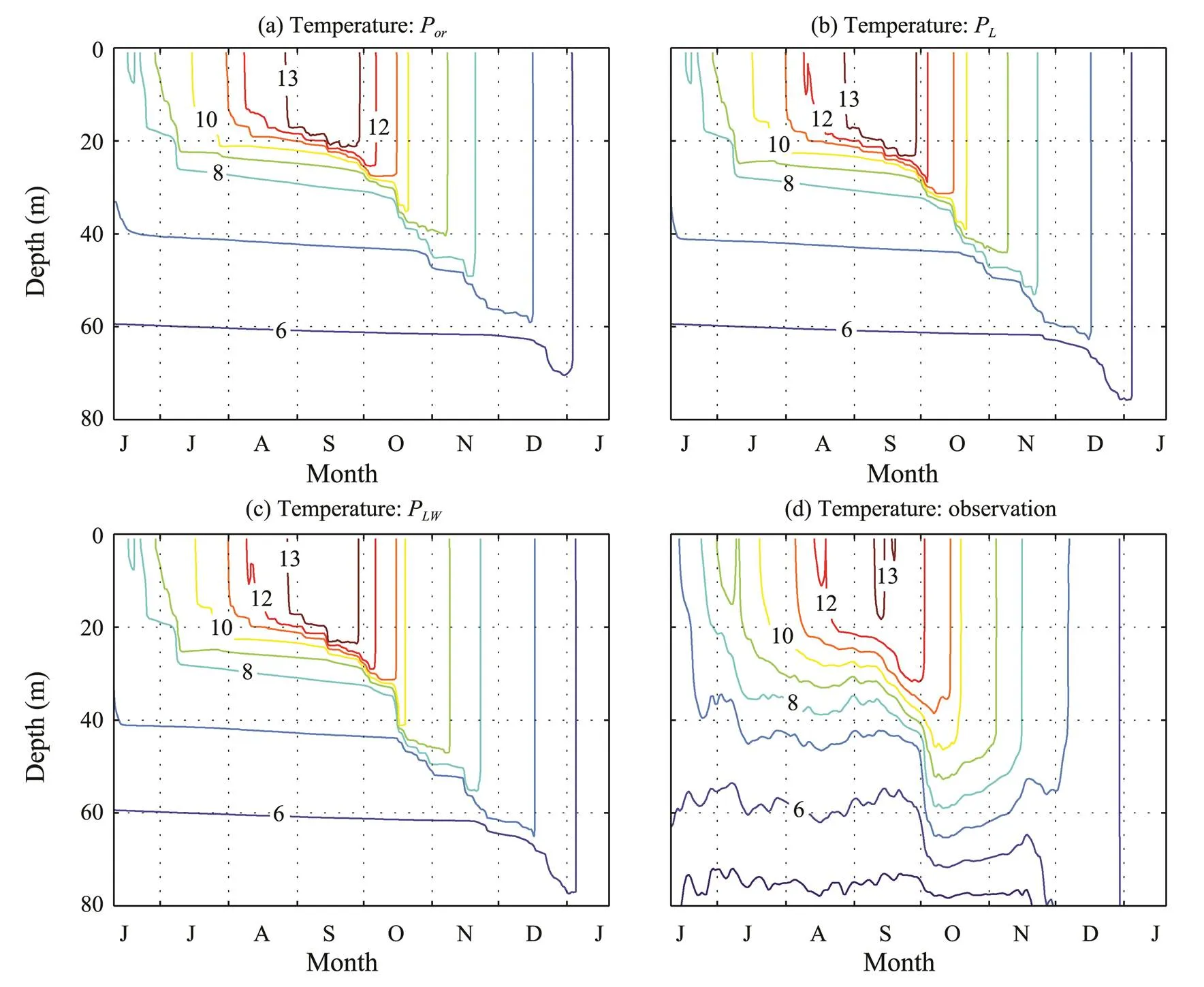
Fig.1 Simulated and observed daily-mean temperature profiles (unit: ℃) at Station Papa from June 2007 to January 2008. (a), Experiment Por; (b), experiment PL; (c), experiment PLW; and (d), field observations. The simulations are based on a one-dimensional model.

The magnitudes of changes in SST and MLD are in accordance with previous studies (Li, 1995; D’Alessio, 1998; Carniel, 2005; Kukulka, 2009; Li, 2013), although most of them argue that LCs play an important role in the upper ocean. For example,D’Alessio(1998)used a similar turbulence closure scheme and observations from Station Papa to show that the maximum change in SST is about 0.2℃ in the cases with and without LC effects. Kukulka(2009) simulated an LC growth event using a LES model in which the change in SST was actually smaller than 0.1℃ although the MLD deepened. In fact, observations by Li(1995) and Kukulka(2009) also showed that changes in SST are actually smaller than 0.1℃ under the effect of LCs.

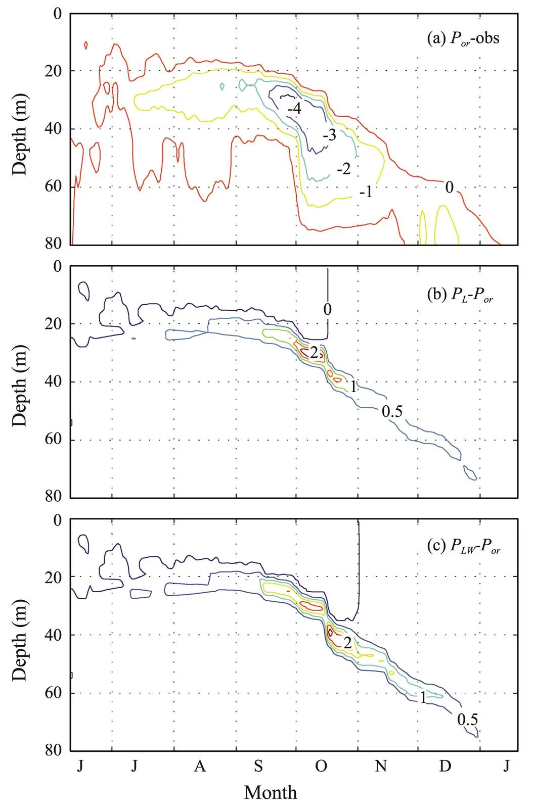
Fig.2 Simulated daily-mean temperature deviations (unit: ℃). (a), Experiment Por minus field observations; (b), experiment PL minus experiment Por; and (c), experiment PLW minus experiment Por. The simulations are based on a one-dimensional model.

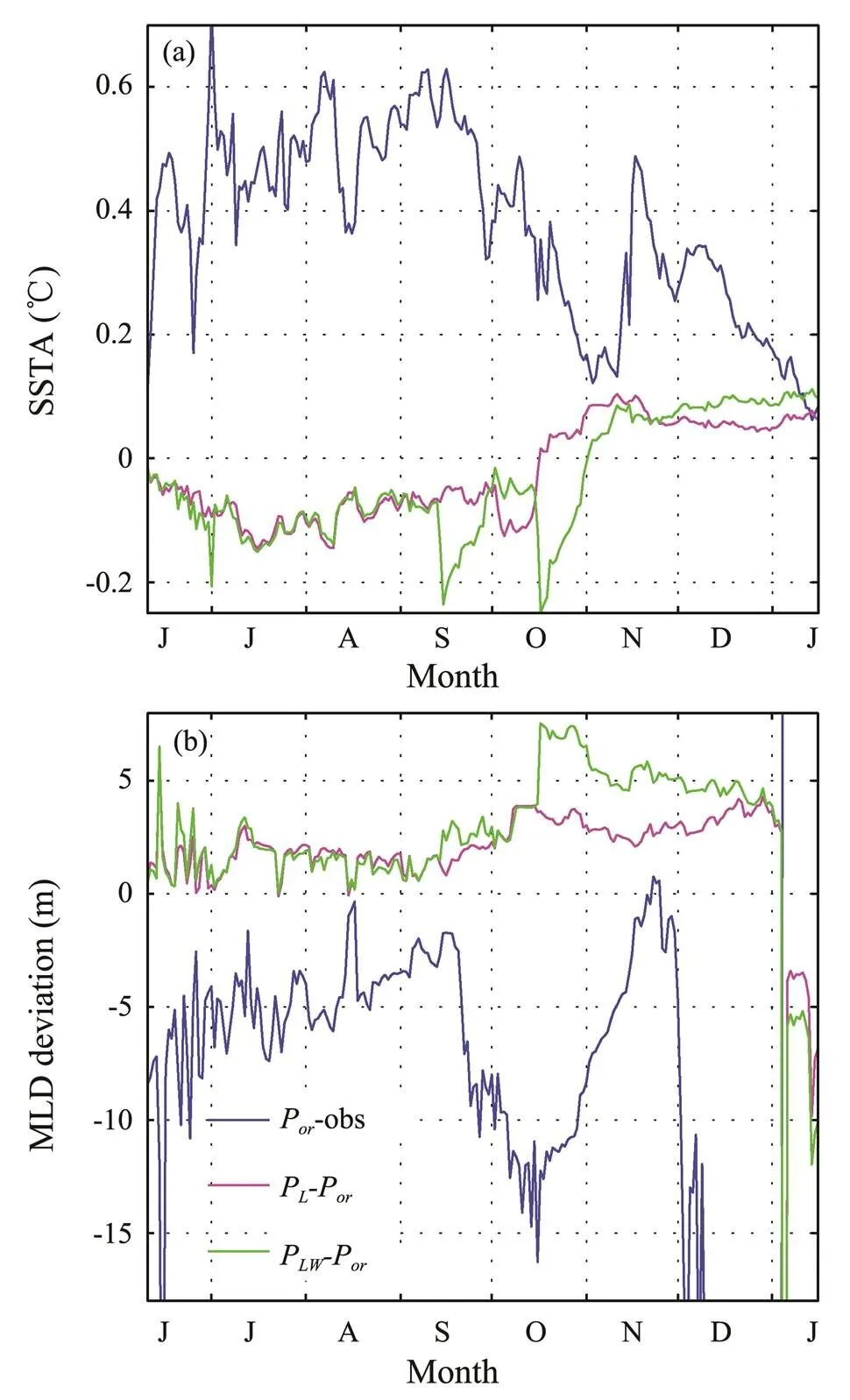
Fig.3 Simulated daily-mean (a) SSTA and (b) MLD deviations between experiment Porand field observations (blue curves), experiment PL and experiment Por(pink curves), and experiment PLW and experiment Por (green curves). MLD is defined as the depth at which the temperature drops by 0.5℃ compared with the surface value. The simulations are based on a one-dimensional model.

Fig.4 shows the simulated daily-mean vertical mixing profiles in experimentPand their deviations from the two other experiments. In these cases, when LCs are incorporated into the model, the simulated vertical mixing is greatly enhanced. However, because these effects are mainly confined to the mixed layer, their ability to regulate the upper-ocean thermal structure is limited.

4 Three-Dimensional Experiments

4.1 Model Description

The behavior of LCs was further assessed by examining simulated subsurface temperatures using the three-dimensional Princeton Ocean model (Blumberg and Mel- lor, 1987). The model domain covers the global ocean between 72˚S and 65˚N with a zonal resolution of 1˚. The meridional resolution is 1/3˚ within 10˚S–10˚N and increases linearly to 1˚ at 20˚N (20˚S). The model includes 32 sigma layers in the vertical direction with at least 6 layers in the top 60m and at least 10 additional levels between 60 and 250m. The bottom topography is obtained from ETOPO5, and the maximum water depth is set to 5000m.

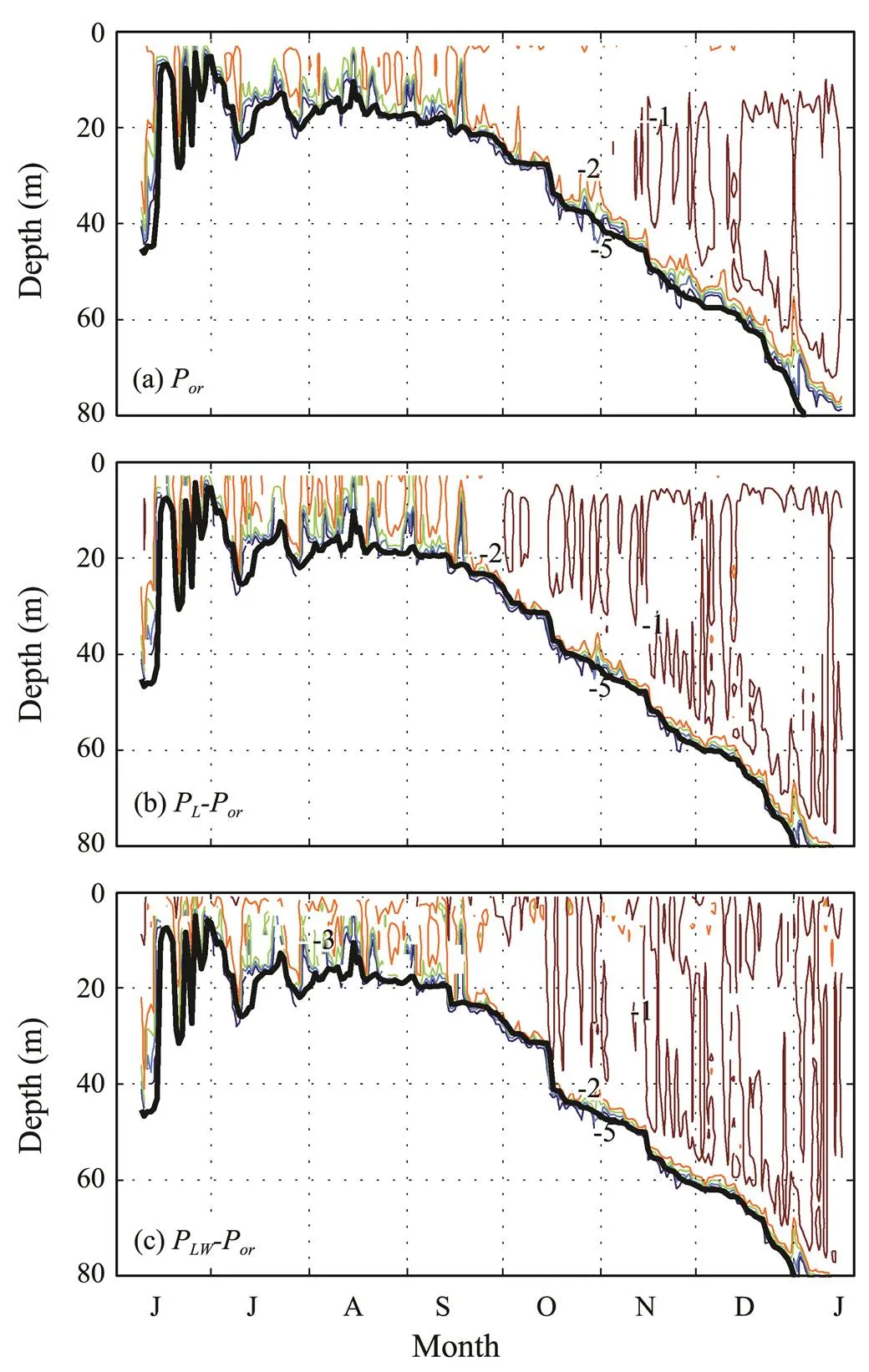
Fig.4 Simulated daily-mean vertical mixing coefficients as a function of depth and time in (a) experiment Por, and their deviations (b) experiment PLminus experiment Por, and (c) experiment PLWminus experiment Por. The denary logarithm of the mixing coefficient (unit: m2 s−1) is shown, and the thick black curve indicates the simulated MLD. The simulations are based on a one-dimensional model.

The model is initiated by using the temperature and salinity conditions in January taken from the WOA01 climatology (Conkright, 2002). The climatological month- ly-mean wind stress is taken from the data of QSCAT/NCEP blended ocean winds from 2000 to 2005 (Milliff, 2004). The surface heat and freshwater fluxes are taken from the monthly-mean COADS climatology (da Silva, 1994). The SST and SSS are relaxed to the monthly-mean WOA01 climatology, with relaxations of 50Wm−2K−1for SST and 60d for SSS (for a MLD of 25m), to prevent surface density values from drifting too far from the climatology. Similar to Section 3, three experiments, named asG,G, andG, were also carried out (Table 1). Each case was integrated for 12 years from a state of rest, and the outputs of the model in the last three years are used to analyze LC effects.

4.2 Results

Fig.5 shows monthly-mean temperature differences along 170˚W in August for the three cases. Vertical mixing from surface waves is more important than that associated with the velocity shear of the mean current in the upper portion of extra-tropical oceans (Noh, 2004; Qiao and Huang, 2012). In experimentG, which does not consider the effects of surface waves, the simulated subsurface temperature is seriously underestimated due to insufficient mixing in the middle latitude between 20˚N and 50˚N when compared with the WOA01 climatological data. The maximum bias can reach up to 3℃ (Fig.5a). The temperature change induced by LC effects alone shows an amplitude of 0.1℃ (Fig.5b) and is consistently negligible in comparison with the large cold bias in experimentG. In experimentG, which considers the com- bined effects of LCs and wave breaking, the subsurface temperature increases greatly due mainly to the effects of wave breaking (Huang, 2011) and shows a maximum value of 2.5℃ (Fig.5c). However, this change is mainly confined to the upper 60m layer; thus, it is insufficient to correct the cold bias in the subsurface layer.

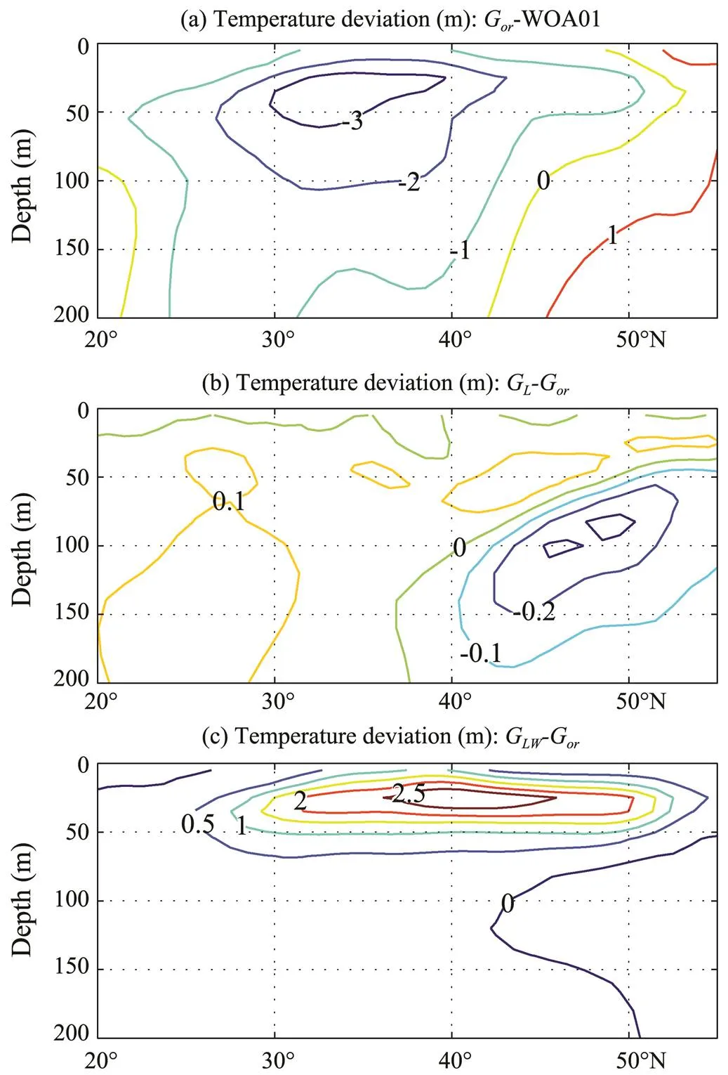
Fig.5 Monthly-meantemperaturedifferences(in℃)along170˚W in August. (a), Experiment Gor minus WOA01; (b),experiment GL minus experiment Gor; and (c), experimentGLW minus experiment Gor. The experiments are based on a three-dimensional model.

The behavior of LCs can also be seen in Fig.6, which shows monthly-mean model temperature errors along 30˚Nin August for the three cases. The cold subsurface bias also results from an unrealistic thermocline (Fig.7). Compared with the WOA01 climatology (Fig.7d), the seasonal thermocline is much shallower and sharper for all three cases.

Fig.8 shows the temperature profiles at the central point of the North Pacific Ocean (30˚N, 170˚W). The effects of LCs are too small to produce significant changes. Compared with experimentG, the simulated temperature seems to slightly increase at a depth of 100–200m in experimentG. In experimentG, the simulated temperature increases further, and the MLD increases remarkably; however, large deviations compared with field observations may still be found.

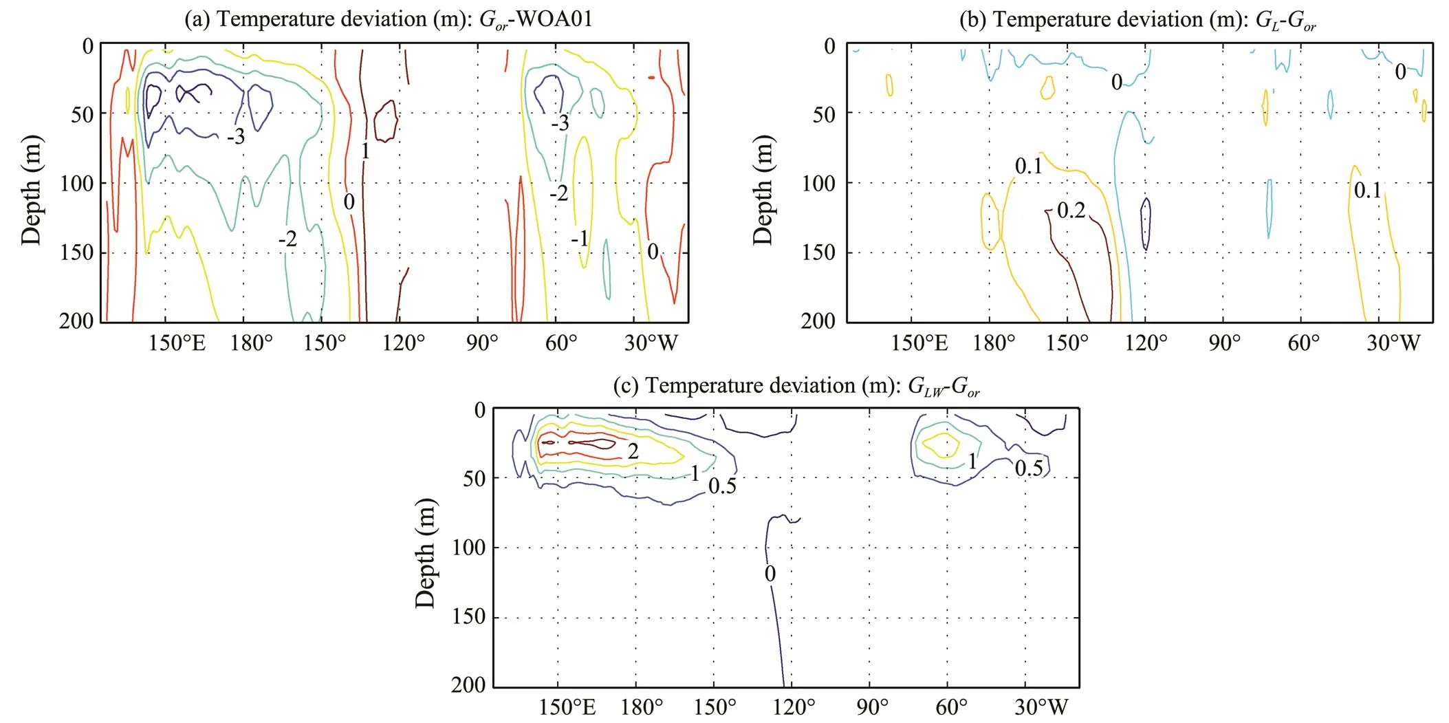
Fig.6 Monthly-mean temperature differences (in ℃) along 30˚N in August. (a), Experiment Gor minus WOA01; (b), experiment GL minus experiment Gor; and (c), experiment GLW minus experiment Gor. The experiments are based on a three-dimensional model.

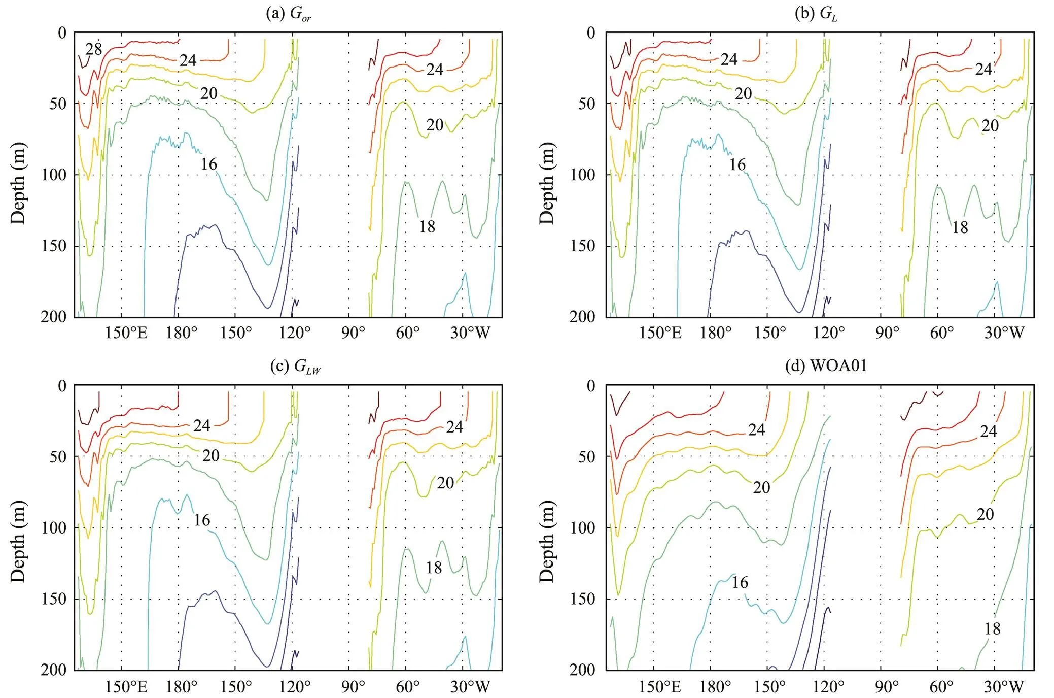
Fig.7 Temperature distribution along 30˚N in August from (a) experiment Gor, (b) experiment GL, (c) experiment GLW, and (d) the WOA01 climatology. The contour interval is 2℃. The experiments are based on a three-dimensional model.

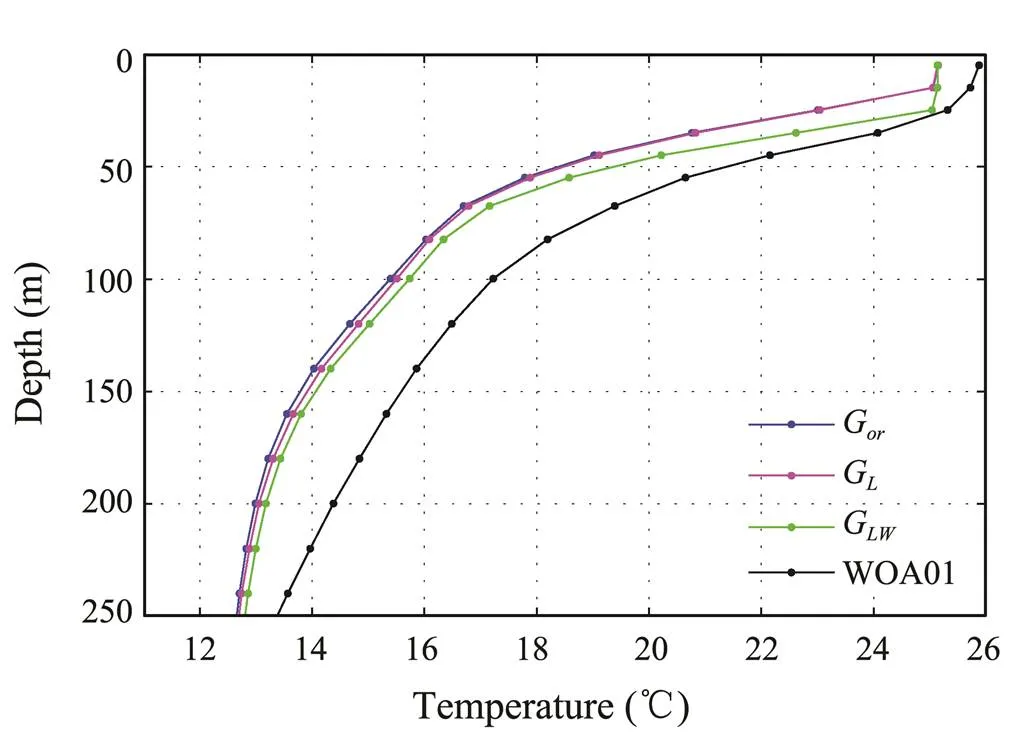
Fig.8 Simulated and climatological monthly-mean temperature profiles in August at 30˚N, 170˚W. The simulations are based on a three-dimensional model.

5 Climate Models

CMIP5 includes most of the state-of-the-art climate models and earth system models; four of the models in thisproject,namely,CNRM-CM5,IPSL-CM5A-LR,IPSL-CM5A-MR, and IPSL-CM5B-LR, consider LC effects (Huang, 2014). In these four models, the scheme of Axell (2002) is used to parameterize effects of LCs (Dufresne, 2013; Voldoire, 2013). In addition, the effects of surface wave breaking are also considered via the scheme of Mellor and Blumberg (2004). The effects of LCs are evaluated by using 20 years (1986–2005) of monthly-averaged outputs from historical runs with an ensemble number of r1i1p1. These historical runs refer to the 20th century simulation forced by observed atmospheric compositional changes, including both natural and anthropogenic sources.

Too-cold subsurface temperatures are a common problem of climate models (Flato, 2013). Fig.9 shows monthly-mean temperature differences along 170˚W in August for these four models in comparison with the WOA01 climatology. All of the models simulate a too-cold upper-ocean temperature. In the near-surface region, the biases of these models deviate by only approximately 1℃ from field observations. This finding implies that the models can well reproduce surface temperatures. However, simulated subsurface temperatures in the middle latitude are seriously underestimated when compared with actual observations. The maximum biases occur at depths between 20 and 60m and are as large as 4℃ in CNRM-CM5 and 7℃ in the three other models. These large biases can also be observed in Fig.10, which shows monthly-mean model temperature errors along 30˚N in August. Similar to our earlier discussion, the cold subsurface bias can be associated with an unrealistic thermocline (Fig.11). Compared with the WOA01 climatology (Fig.7d), the simulated thermoclines are clearly much shallower and sharper in these four models.

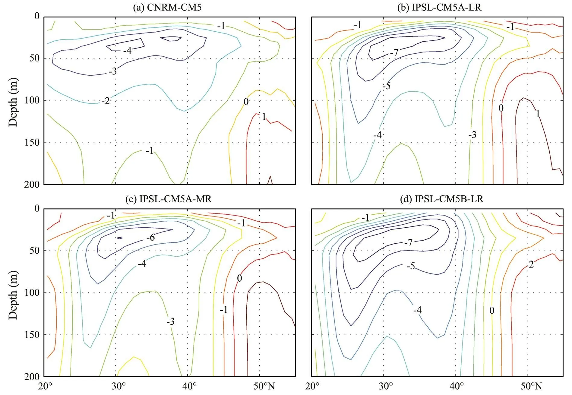
Fig.9 Monthly-mean temperature differences (in ℃) from the WOA01 climatology along 170˚W in August. (a), CNRM-CM5; (b), IPSL-CM5A-LR; (c), IPSL-CM5A-MR; and (d), IPSL-CM5B-LR. The data are obtained from CMIP5 climate models.

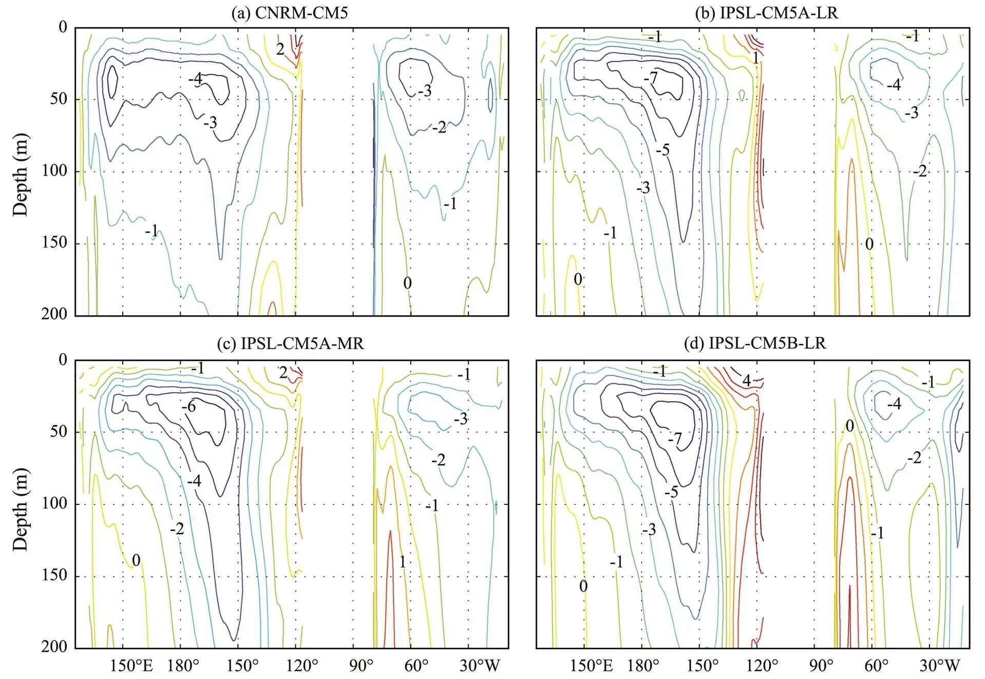
Fig.10 Monthly-mean temperature differences (in ℃) from the WOA01 climatology along 30˚N in August. (a), CNRM-CM5; (b), IPSL-CM5A-LR; (c), IPSL-CM5A-MR; and (d), IPSL-CM5B-LR. The data are obtained from CMIP5 climate models.

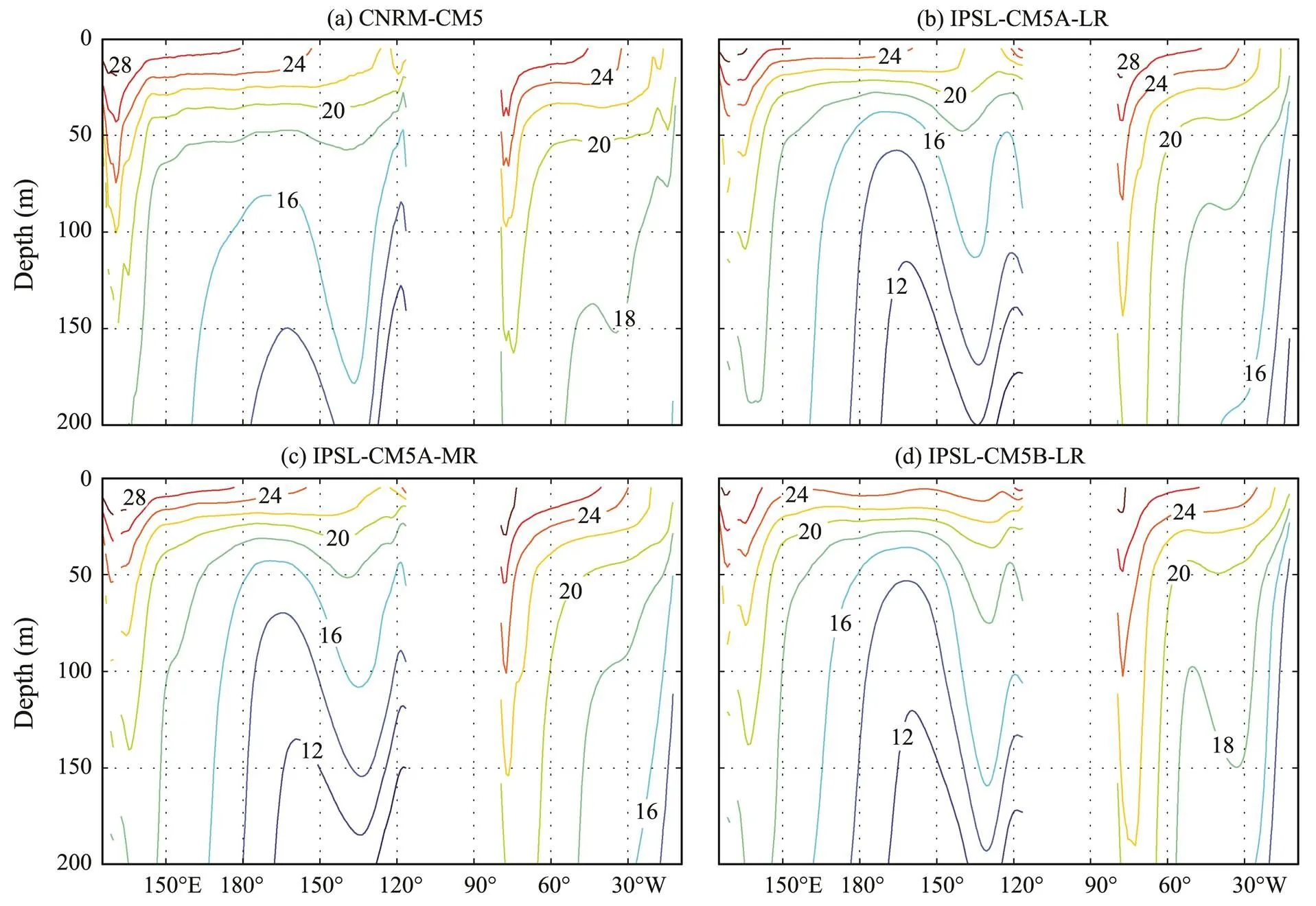
Fig.11 Temperature distribution along 30˚N in August determined from (a) CNRM-CM5, (b) IPSL-CM5A-LR, (c) IPSL-CM5A-MR, and (d) IPSL-CM5B-LR. The contour interval is 2℃. The data are obtained from CMIP5 climate models.

Due to the cold subsurface temperature, summer MLDs are significantly underestimated in the four models, especially in the central North Pacific and Atlantic Oceans (Fig.12 or Huang, 2014). This finding is similar to those of Fan and Griffies (2014) and D’Asaro(2014), who showed that the effects of LCs are insignificant to increases in MLD in summer.

In fact, although LCs can rapidly destroy near-sur- face stratification and increase the MLD (Li, 1995; Kukulka, 2009), their effects seem to be mostly confined to the initial stages of MLD growth (Skyllingstad, 2000). Noh(2011) argued that LCs could significantly increase the MLD only if the latter is shallow and the buoyancy jump across the mixed layer is small. Field observations by Weller and Price (1988) showed that the effects of LCs are confined to the upper part of the mixed layer, insignificant in the lower part, and absent in the relict mixed layer during summer-like conditions or deeper mixed layer during stormy conditions.

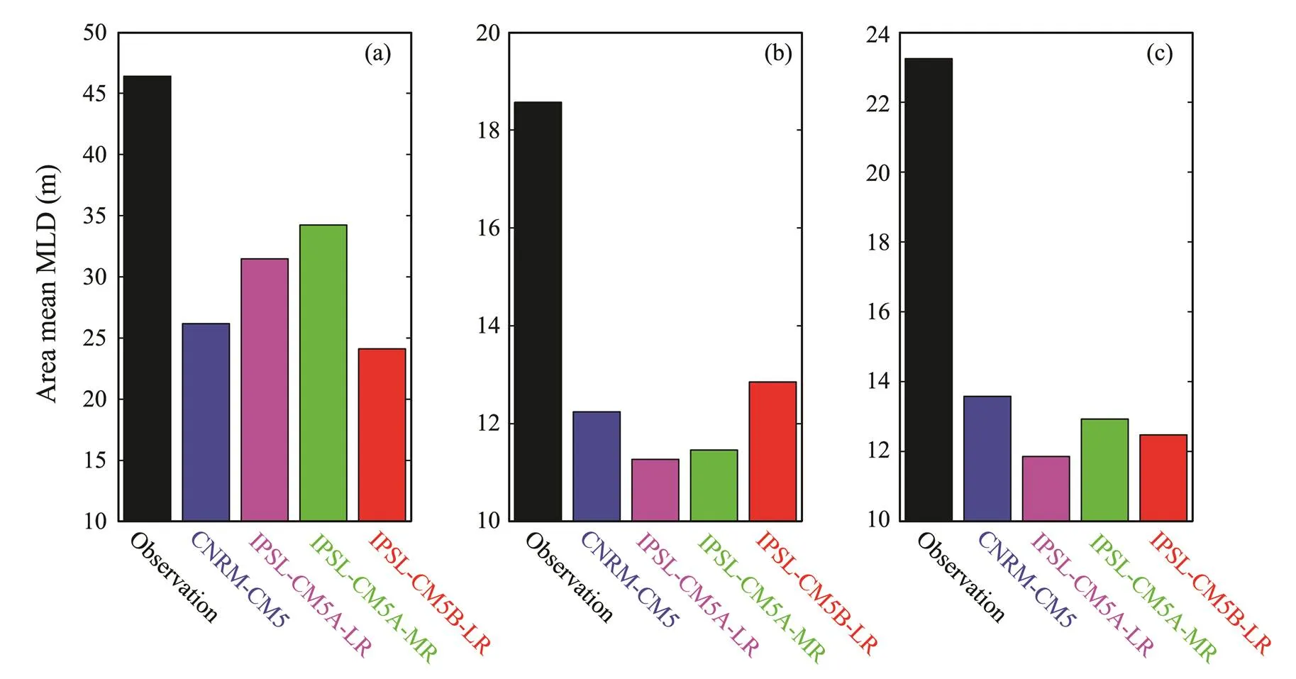
Fig.12 Area-averaged MLDs (a) in austral summer in the Southern Ocean (between 30˚S and 65˚S), (b) in boreal summer in the central Northern Pacific Ocean (35˚S–55˚S, 160˚E–140˚W), and (c) in boreal summer in the central Northern Atlantic (40˚S–65˚S, 50˚W–10˚W) determined from four CMIP5 climate models and field observations. MLD is defined as the depth in which the potential density deviates by 0.03kgm−3 from its value at 10m. The observed MLDs are taken from the climatological monthly MLD data of de Boyer Montégut et al. (2004).

6 Discussion and Conclusions

In this paper, the influences of LCs on the upper-ocean thermal structure are examined by using one- and three-dimensional ocean circulation models, as well as four climate models from the CMIP5. The results show that LCs can slightly improve simulations of MLD and SST in the models; however, their effect on the upper ocean is not sufficiently large to produce significant changes. The models evaluated in this work, including those considering LC effects alone and the combined effects of LCs and wave breaking, failed to produce a reasonable summertime thermocline, resulting in a large cold bias in the subsurface layer. A cold bias is a typical feature induced by insufficient vertical mixing in the upper ocean. Our findings imply that LCs are insufficient to solve the problem of insufficient vertical mixing and that restriction of non-breaking surface wave-induced mixing in LCs may be questionable.

In this study, only two early parameterization schemes of LCs,, those of Kantha and Clayson (2004) and Axell (2002), were analyzed. LCs were studied extensively with LES in the past, and many new schemes have since been proposed. However, the performances of LCs in these new schemes are very similar as those in the present study. Although all researchers claim that their schemes can enhance the vertical mixing of the upper ocean and produce significantly improved simulations of MLD and SST, the improvements observed are, in fact, very limited and large deviations are still recorded. For example, Ali(2019; see their Table 2) investigated the performances of five LC schemes, including those of McWilliams and Sullivan (2000), Smyth(2002), Takaya(2010), Van Roekel(2012), and Li and Fox-Kemper (2017), by using a numerical model of the North Atlantic and Arctic Oceans and found that mean MLDs during summer increase from 4.2% to 14.6% in the model domain south of 50˚Nrelative to the case without wave effects.

Our conclusions are only based on numerical model results, which depend on the behaviors of the models and the parameterization of LCs used. Therefore, further stud- ies, especially those involving field observations, are need- ed to comprehensively understand the effects of LCs on the upper ocean.In addition, studying non-breaking surface wave-induced mixing from a more comprehensive perspective (Veron, 2009; Ghantous and Babanin, 2014; Qiao, 2016), rather than LCs alone, is necessary to simulate the upper ocean accurately.

Acknowledgements

Data of the CMIP5 models are available at https://esgf-data.dkrz.de/search/cmip5-dkrz/. CJH and DD were supported by the National Key Research and Development Program of China (No. 2017YFC1404000), the Basic Scientific Fund for National Public Research Institutes of China (No. 2018S03), and the National Natural Science Foundation of China (Nos. 41776038 and 41376036). Dr. Fangli Qiao was supported by the Natural Science Founda- tion of China (Nos. 41821004).

Agrawal, Y. C., Terray, E. A., Donelan, M. A., Hwang, P. A., Williams III, A. J., Drennan, W. M., Kahma, K. K., and Kitaigorodskii, S. A., 1992. Enhanced dissipation of kinetic energy beneath surface waves., 359: 219-220.

Ali, A., Christensen, K. H., Breivik, Ø., Malila, M., Raj, R. P., Bertino, L., Chassignet, E. P., and Bakhoday-Paskyabi, M., 2019. A comparison of Langmuir turbulence parameterizations and key wave effects in a numerical model of the North Atlantic and Arctic Oceans., 137: 76-97.

Anis, A., and Moum, J. N., 1995. Surface wave-turbulence interactions: Scaling() near the sea surface., 25: 2025-2045.

Axell, L. B., 2002. Wind-driven internal waves and Langmuir circulations in a numerical ocean model of the southern Baltic Sea., 107 (C11): 3204, DOI: 10.1029/2001JC000922.

Belcher, S. E., Grant, A. L. M., Hanley, K. E., Fox-kemper, B., Roekel, L. V., Sullivan, P. P., Large, W. G., Brown, A., Hines, A., Calvert, D., Rutgersson, A., Pettersson, H., Bidlot, J.-R., Janssen, P. A. E. M., and Polton, J. A., 2012. A global perspective on Langmuir turbulence in the ocean surface boundary layer., 39: L18605, DOI: 10.1029/2012GL052932.

Blumberg, A. F., and Meller, G. L., 1987. A description of a three-dimensional coastal ocean circulation model. In:(Chapter 4)Heaps, N. S., ed., American Geophysical Union, Washington, D.C., 1-16.

Carniel, S., Sclavo, M., Kantha, L. H., and Clayson, C. A., 2005. Langmuir cells and mixing in the upper ocean., 28: 33-54.

Conkright, M. E., Locarnini, R. A., Garcia, H. E., O’Brien, T., Boyer, T. P., Stephens, C., and Antonov, J. I., 2002.. National Oceanographic Data Center, Silver Spring, MD, Internal Report 17, 17pp.

Craig, P. D., and Banner, M. L., 1994. Modeling wave-enhanced turbulence in the ocean surface layer., 24: 2546-2559.

D’Alessio, S. J. D., Abdella, K., and McFarlane, N. A., 1998. A new second-order turbulence closure scheme for modelling the ocean mixed layer., 28: 1624-1641.

D’Asaro, E. A., Thomson, J., Shcherbina, A. Y., Harcourt, R. R., Cronin, M. F., Hemer, M. A., and Fox-Kemper, B., 2014. Quantifying upper ocean turbulence driven by surface waves., 41: 102-107, DOI: 10.1002/2013GL058193.

da Silva, A., Young, A. C., and Levitus, S., 1994.. NOAA Atlas NESDIS 6, U.S. Department of Commerce, Washington, D.C., 83pp.

de Boyer Montégut, C., Madec, G., Fischer, A. S., Lazar, A., and Iudicone, D., 2004. Mixed layer depth over the global ocean: An examination of profile data and a profile-based climatology., 109: C12003, DOI: 10.1029/2004JC002378.

Donelan, M. A., 1998. Air-water exchange processes. In:(Chapter 2)Imberger, J., ed., American Geophysical Union, Washington, D.C., 19-36.

Drennan, W. M., Donelan, M. A., Terray, E. A., and Katsaros, K. B., 1996. Oceanic turbulence dissipation measurements in SWADE., 26: 808-815.

Dufresne, J.-L., Foujols, M.-A., Denvil, S., Caubel, A., Marti, O., Aumont, O., Balkanski, Y., Bekki, S., Bellenger, H., Benshila, R., Bony, S., Bopp, L., Braconnot, P., Brockmann, P., Cadule, P., Cheruy, F., Codron, F., Cozic, A., Cugnet, D., de Noblet, N., Duvel, J.-P., Ethé, C., Fairhead, L., Fichefet, T., Flavoni, S., Friedlingstein, P., Grandpeix, J.-Y., Guez, L., Guilyardi, E., Hauglustaine, D., Hourdin, F., Idelkadi, A., Ghattas, J., Joussaume, S., Kageyama, M., Krinner, G., Labetoulle, S., Lahellec, A., Lefebvre, M.-P., Lefevre, F., Levy, C., Li, Z. X., Lloyd, J., Lott, F., Madec, G., Mancip, M., Marchand, M., Masson, S., Meurdesoif, Y., Mignot, J., Musat, I., Parouty, S., Polcher, J., Rio, C., Schulz, M., Swingedouw, D., Szopa, S., Talandier, C., Terray, P., Viovy, N., and Vuichard, N., 2013. Climate change projections using the IPSL-CM5 Earth System Model: From CMIP3 to CMIP5., 40: 2123-2165, DOI: 10/1007/s00382-012-1636-1.

Ezer, T., 2000. On the seasonal mixing layer simulated by a basin-scale ocean model and the Mellor-Yamada turbulence scheme., 105: 16843-16855.

Fan, Y., and Griffies, S. M., 2014. Impacts of parameterized Langmuir turbulence and non-breaking wave mixing in global climate simulations., 27: 4752-4775.

Flato, G., Marotzke, J., Abiodun, B., Braconnot, P., Chou, S. C., Collins, W., Cox, P., Driouech, F., Emori, S., Eyring, V., Forest, C., Gleckler, P., Guilyardi, E., Jakob, C., Kattsov, V., Reason, C., and Rummukainen, M., 2013. Evaluation of climate models. In:. Stocker, T. F.,, eds., Cambridge University Press, Cambridge, United Kingdom and New York, NY, 741-866.

Gemmrich, J. R., and Farmer, D. M., 2004. Near-surface turbulence in the presence of breaking waves., 34: 1067-1086.

Ghantous, M., and Babanin, A. V., 2014. Ocean mixing by wave orbital motion., 64 (1): 1-56.

Grant, A. L. M., and Belcher, S. E., 2009. Characteristics of Langmuir turbulence in the ocean mixed layer., 39: 1871-1887.

Harcourt, R. R., 2013. A second-moment closure model of Langmuir turbulence., 43: 673-697, DOI: 10.1175/JPO-D-12-0105.1.

Huang, C. J., Qiao, F. L., and Dai, D. J., 2014. Evaluating CMIP5 simulations of mixed layer depth during summer.,119:2568-2582,DOI:10.1002/2013JC009535.

Huang, C. J., Qiao, F. L., Song, Z. Y., and Ezer, T., 2011. Improving simulations of the upper ocean by inclusion of surface waves in the Mellor-Yamada turbulence scheme., 116: C01007, DOI: 10.1029/2010JC006320.

Kantha, L. H., and Clayson, C. A., 2004. On the effect of surface gravity waves on mixing in the oceanic mixed layer., 6: 101-124.

Kantha, L. H., Lass, U., and Prandke, H., 2010. A note on Stokes production of turbulence kinetic energy in the oceanic mixed layer: Observations in the Baltic Sea., 60: 171-180, DOI: 10.1007/s10236-009-0257-7.

Kukulka, T., Plueddemann, A. J., Trowbridge, J. H., and Sullivan, P. P., 2009. Significance of Langmuir circulation in upper ocean mixing: Comparison of observations and simulations., 36: L10603, DOI: 10.1029/2009GL037620.

Large, W. G., McWilliams, J. C., and Doney, S. C., 1994. Oceanic vertical mixing: A review and a model with a nonlocal boundary layer parameterization., 32: 363-403.

Leibovich, S., and Paolucci, S., 1980. The Langmuir circulation instability as a mixing mechanism in the upper ocean., 10: 186-207.

Li, M., and Garrett, C., 1997. Mixed layer deepening due to Langmuir circulation., 27: 121-132.

Li, M., Zahariev, K., and Garrett, C., 1995. Role of Langmuir circulation in the deepening of the ocean surface mixed layer., 270 (5244): 1955-1957.

Li, Q., and Fox-Kemper, B., 2017. Assessing the effects of Langmuir turbulence on the entrainment buoyancy flux in the ocean surface boundary layer.,47 (12): 2863-2886.

Li, Q., Webb, A., Fox-Kemper, B., Craig, A., Danabasoglu, G., Large, W. G., and Vertenstein, M., 2016. Langmuir mixing effects on global climate: WAVEWATCH III in CESM., 103: 145-160.

Li, S., Song, J., and Fan, W., 2013. Effect of Langmuir circulation on upper ocean mixing in the South China Sea., 32 (3): 28-33, DOI: 10.1007/s13131-013-0285-5.

Martin, P. J., 1985. Simulation of the mixed layer at OWS November and Papa with several models., 90: 581-597.

McWilliams, J. C., and Sullivan, P. P., 2000. Vertical mixing by Langmuir circulations., 6: 225-237.

McWilliams, J. C., Sullivan, P. P., and Moeng, C.-H., 1997. Langmuir turbulence in the ocean., 334: 1-33.

Mellor, G., and Blumberg, A., 2004. Wave breaking and ocean surface layer thermal response., 34: 693-698.

Mellor, G., and Yamada, T., 1982. Development of a turbulence closure model for geophysical fluid problems., 20: 851-875.

Milliff, R. F., Morzel, J., Chelton, D. B., and Freilich, M. H., 2004. Wind stress curl and wind stress divergence biases from rain effects on QSCAT surface wind retrievals., 21: 1216-1231.

Noh, Y., 2004. Sensitivity to wave breaking and the Prandtl number in the ocean mixed layer model and its dependence on latitude., 31: L23305, DOI: 10.1029/2004GL021289.

Noh, Y., Goh, G., and Raasch, S., 2011. Influence of Langmuir circulation on the deepening of the wind-mixed layer., 41: 472-484, DOI: 10.1175/2010JPO4494.1.

Noh, Y., Min, H. S., and Raasch, S., 2004. Large eddy simulation of the ocean mixed layer: The effects of wave breaking and Langmuir circulation., 34: 720-735.

Phillips, O. M., 1961. A note on the turbulence generated by gravity waves., 66: 2889-2893.

Qiao, F. L., and Huang, C. J., 2012. Comparison between vertical shear mixing and surface wave-induced mixing in the extratropical ocean., 117: C00J16, DOI: 10.1029/2012JC007930.

Qiao, F. L., Yuan, Y. L., Deng, J., Dai, D. J., and Song, Z. Y., 2016. Wave-turbulence interaction-induced vertical mixing and its effects in ocean and climate models., 374: 20150201, http://dx.doi.org/10.1098/rsta.2015.0201.

Rapp, R. J., and Melville, W. K., 1990. Laboratory measurements of deep-water breaking waves., A331: 735-800.

Skyllingstad, E. D., Smyth, W. D., and Crawford, G., 2000. Resonant wind driven mixing in the ocean boundary layer., 30: 1866-1890.

Skyllingstad, E., and Denbo, D., 1995. An ocean large-eddy simu- lation of Langmuir circulations and convection in the surface mixed layer., 100: 8501-8522.

Smyth, W. D., Skyllingstad, E. D., Crawford, G. B., and Wijesekera, H., 2002. Nonlocal fluxes and stokes drift effects in the K-profile parameterization., 52: 104-115.

Soloviev, A., and Lukas, R., 2006.. Springer, Dordrecht, Netherlands, 572pp.

Soloview, A., and Lukas, R., 2003. Observation of wave-enhanced turbulence in the near-surface layer of the ocean during TOGA COARE., 50: 371-395.

Sullivan, P. P., McWilliams, J. C., and Melville, W. K., 2007. Surface gravity wave effects in the oceanic boundary layer: Large-eddy simulation with vortex force and stochastic breakers., 593: 405-452.

Takaya, Y., Bidlot, J.-R., Beljaars, A. C. M., and Janssen, P. A. E. M., 2010. Refinements to a prognostic scheme of skin sea surface temperature., 115: C06009, DOI: 10.1029/2009JC005985.

Taylor, K. E., Stouffer, R. J., and Meehl, G. A., 2012. An overview of CMIP5 and the experiment design., 93: 485-498.

Van Roekel, L. P., Fox-Kemper, B., Sullivan, P. P., Hamlington, P. E., and Haney, S. R., 2012. The form and orientation of Langmuir cells for misaligned winds and waves.,117 (C5): C05001, DOI: 10.1029/2011JC007516.

Veron, F., Melville, W. K., and Lenain, L., 2009. Measurements of ocean surface turbulence and wave-turbulence interactions., 39: 2310-2323.

Voldoire, A., Sanchez-Gomez, E.,Salasy Mélia, D.,Decharme, B.,Cassou, C.,Sénési, S., Valcke, S.,Beau, I., Alias, A.,Chevallier, M.,Déqué, M., Deshayes, J., Douville, H., Fernandez, E., Madec, G.,Maisonnave, E.,Moine, M.-P., Planton, S.,Saint-Martin, D., Szopa, S.,Tyteca, S., Alkama,R., Belamari,S.,Braun, A.,Coquart, L., and Chauvin, F., 2013. The CNRM-CM5.1 global climate model: Description and basic evaluation., 40: 2091-2121, DOI: 10.1007/s00382-00011-1259-y.

Weller, R. A., and Price, J. F., 1988. Langmuir circulation within the oceanic mixed layer., 35 (5): 711-747.

Young, I. R., and Babanin, A. V., 2006. Spectral distribution of energy dissipation of wind-generated waves due to dominant wave breaking., 36: 376-394.

Zhang, S., Yuan, Y., and Zheng, Q., 2007. Modeling of the eddy viscosity by breaking waves., 26 (6): 116-123.

. Tel: 0086-532-88961709

E-mail: djdai@fio.org.cn

September 4, 2019;

December 4, 2019;

January 3, 2020

(Edited by Xie Jun)