Active micro-vibration control based on improved variable step size LMS algorithm ①

Li Xiangmin(李相敏), Fang Yubin, Zhu Xiaojin , Huang Yonghui, Zhou Yijia

(School of Mechatronics Engineering and Automation,Shanghai University, Shanghai 200240, P.R.China)

Abstract

Key words: adaptive filtering, variable step size least mean square (LMS) algorithm, logarithmic and symbolic functions, convergence and steady state error, active control of micro vibration

0 Introduction

Adaptive filtering is an optimal filtering method developed on the basis of Wiener filtering and Kalman filtering[1]. Due to its stronger adaptability and better filtering performance, it has been widely used in engineering practice, especially information processing technology field. The least mean square (LMS) algorithm is a stochastic gradient algorithm and an adaptive filter. It has the advantages of small computation, strong robustness and easy engineering implementation. It is widely used in system identification, adaptive equalization, noise cancellation, active vibration control and other fields[2,3]. In LMS algorithm, convergence speed, tracking speed, steady-state error and steady-state misalignment are the main technical indicators to measure the performance of LMS algorithm[4].

The step factor of fixed step size LMS algorithm is invariable; the algorithm can not meet the requirements of fast convergence speed and small steady-state error at the same time. In the research of active control of micro-vibration, it is hoped that the algorithm will have large step-size factor to accelerate convergence in the initial stage and reduce steady-state in the later stage. In order to solve this contradiction further, a variety of variable step size LMS algorithms based on a fixed step size are proposed.

The difference between these algorithms is the way in which the step size is updated. Some algorithms get the current step size by modifying the previous step size, while others adjust the step size through a non-linear function. In Ref.[5], a variable step size LMS algorithm based on Sigmoid was proposed. It not only has better convergence and tracking performance, but also can obtain smaller steady-state error. Nevertheless, the function Sigmoid changes too fast when the error tends to zero, which makes the algorithm still have a large step in steady state, thus increasing the steady-state error of steady-state misalignment. Based on this, an improved algorithm was proposed in Ref.[6], which makes the step size of the algorithm in steady state very small, and solves the defect of Ref.[6] to a certain extent. A variable step size LMS algorithm based on probability function was proposed in Ref.[6]. Although it can obtain faster convergence speed, tracking speed, and smaller steady-state error and steady-state misalignment simultaneously. However, in the special environment, the convergence speed, tracking speed and steady-state error of the algorithm are not ideal. In Ref.[7], a variable step size LMS algorithm based on genetic algorithm was proposed. The algorithm has better convergence speed and tracking speed, and can get smaller steady-state mean square error. However, when the algorithm reaches steady-state, the instantaneous error will increase if the parameters of the system are changed. In Ref.[8], a new variable step size LMS algorithm was proposed, and a new non-linear function relationship between step size factor and error is established by arctan function. A new variable step size LMS algorithm is presented. In Ref.[9], a VSS-LMS (variable step size LMS) algorithm was proposed, which normalizes the reference signal, enhances the anti-interference ability of the algorithm and reduces the steady-state error of the algorithm after convergence. However, the convergence speed of the algorithm is also slow because of the slow change of the step factor in the earlier stage of the algorithm. In Ref.[10], in order to reduce the impact caused by the sudden change of reference signal and error signal, the step factor was correlated with them, but the convergence speed of the algorithm is also weakened. In Ref.[11], in order to prevent overshoot of step factor updating, adjusting parameters was introduced to further enhance the anti-jamming ability, but the convergence speed of the algorithm in the early stage lagged behind, and it cannot converge to a small steady-state error in a short time.

Based on the characteristics and shortcomings of variable step size LMS algorithm in the previous literature, a variable step size algorithm is proposed based on the combination of logarithmic function and symbolic function. The proposed algorithm not only guarantees small steady-state error, but also improves the convergence speed of the variable step size algorithm in the initial stage[12]. That is, the algorithm has a large step factor to accelerate convergence when the error signal is large, and a small step factor to reduce steady-state error after convergence.

1 Principle of LMS adaptive filtering algorithm

The main idea of adaptive filtering is to apply the same size and opposite direction control output to the disturbance source, to achieve the vibration suppression of the controlled object[13,14]. Fig.1 is the basic principle of adaptive filtering. The filter compares the input signal processing with the desired signal, and then feeds back the performance data of the adaptive algorithm to the filter. The filter parameters are adjusted to make the output tend to the desired signal.

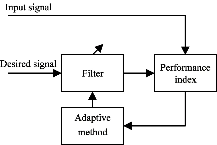
Fig.1 Basic principles of adaptive filtering control

Among many adaptive algorithms, least mean square algorithm is widely used, because of its good convergence, small computation and strong tracking ability. The step size of LMS algorithm affects its convergence speed and steady-state error, which directly affects the performance of the algorithm. Therefore, the step factor of variable step size algorithm is of great significance for improving LMS algorithm[15]。

The step factor of LMS algorithm plays a key role in the performance of filtered-X LMS (FXLMS) algorithm[16,17]. The rule of step size selection can be summarized as follows: large step size factor satisfies the characteristics of fast adaptive convergence, but will produce excessive mean square error (EMSE). If the step size is too large, the system may lose the stability. On the other hand, too small step size will lead to slow convergence speed of system. Even if the mean square error is small, it cannot be accepted by many practical applications. Therefore, in order to ensure that the experiment of active micro-vibration control has a good effect, determining the appropriate step size is an important research content of LMS adaptive filtering algorithm.

2 Modified variable step size LMS algorithm

According to the law of adjusting step size, the algorithm can be grouped into 3 categories: one is the correlation between step size adjustment and input signal, the other is the correlation between step size adjustment formula and error signal, and the third is the correlation between step size adjustment formula and error signal at the same time. The rule of step size change of variable step size algorithm is: always hoping to have a large step size in the initial stage to accelerate convergence; after convergence, the algorithm has a small step size to ensure a small steady-state error.

Ref.[9] proposed a VSS-LMS algorithm in 1988 and gave its simplified version in 1990. The updated formulas are

(1)

ρ(n)=(1-λ)x(n-1)e(n-1)+λ(n-1)

(2)

Ref.[10] proposed a VSS-LMS algorithm in 1990. The updating formulas of step factor are

μ(n)=μ(n-1)+αe(n)xT(n)η(n)

(3)

η(n+1)=η(n)-μ(n)x(n)xT(n)η(n)

+x(n)e(n)

(4)

The condition that the step size factor satisfies is

(5)

The parameters that need to be adjusted in the above algorithm areα,μmaxandμmin, whereμmaxandμminare the upper and lower limits of step size factor. Andαis the factor, whose values are usually small positive numbers. The step factor updating formula correlates the error signal with the input signal, which enhances anti-interference ability of the algorithm and reduces the influence caused by the signal mutation. However, because the step factor follows the error signal linearly, it cannot get a larger value in the initial operation of the algorithm, which results in the poor convergence rate in the initial operation of the algorithm.

Ref.[11] proposed another VSS-LMS algorithm in 2005. The update formulas of step size are

(6)

(7)

In order to overcome the shortcomings of the above algorithm, logarithmic function and symbolic function are introduced to accelerate its convergence speed.To enhance the anti-jamming ability, the input signal is normalized and the step size is correlated with the input signal and the error signal. Thex(n-1) input signal in the modification (2) is replaced by sign(x(n-1)). After introducing symbolic function, the value of input signal changes to -1, 0 or 1, which accelerates the convergence speed of the algorithm in the initial stage and reduces the risk of overshoot. Since the introduction of symbolic function increases the jumping property of the algorithm value, the anti-jumping parameterβis added to the formula to reduce the steady-state error and the steady-state misalignment. At this point,ρ(n) becomes:

ρ(n)=(1-λ)βsign(x(n-1))e(n-1)

+λ(n-1)

(8)

After these improvements, the steady-state error of parameterβis greatly reduced, but the convergence speed of initial stage is weakened. For enhancing the convergence ability of the algorithm in the initial stage further, the error signale(n-1) in the modification (2) is replaced by ln(1-|e(n-1)|). At the initial stage of the algorithm, the error signale(n-1) is larger, while the value of 1-|e(n-1)| becomes a very small number between 0 and 1.When the value of 1-|e(n-1)| approaches 0, the value of ln(1-|e(n-1)|) will become smaller. The larger the value ofρ(n), the larger the step factorμ(n). Therefore, the initial convergence speed of the algorithm is greatly accelerated. When the algorithm converges quickly, the value of error signale(n-1) decreases and the value of 1-|e(n-1)| approaches 1, so the value of ln(1-|e(n-1)|) decreases and tends to zero. Furthermore, it ensures that the algorithm has small step size factor, steady-state error and steady-state misalignment after convergence. At this point,ρ(n) becomes the following:

ρ(n)=(1-λ)βsign(x(n-1))ln(1-|e(n-1)|)

+λρ(n-1)

(9)

In the initial stage, due to the large error signale(n-1), the value of ln(1-|e(n-1)|) tends to be negative infinite, and there cannot be infinite value in the operation of the algorithm. Therefore, on the basis of the above, a lower limit factor constantδminis added to limit the value of ln(1-|e(n-1)|). The order is the following:

δ=ln(1-|e(n-1)|)

(10)

So far, the variable step size LMS algorithm based on logarithmic and symbolic functions is summarized as

e(n)=d(n)-y(n)

(11)

(12)

ρ(n)=(1-λ)βsign(x(n-1))

ln(1-|e(n-1)|)+λρ(n-1)

(13)

δ=δmin, ifδ<δmin

(14)

w(n+1)=w(n)+μ(n)e(n)x(n)

(15)

Among them,w(n) is the weight vector of the adaptive filter;x(n) is the tap input signal vector of the adaptive filter;e(n) is the error signal;μ(n) is the step factor;y(n) is the output signal;d(n) is the expected signal;φis the scaling factor;λis the forgetting factor, and its range is [0.9,1];δminis constant.

3 Performance analysis of improved variable step size LMS algorithm

3.1 Convergence analysis of algorithms

The convergence factorμ(n) in variable step size LMS algorithm determines the updating quantity of tap weight vector in each iteration, which is a key parameter affecting the convergence speed of the algorithm. Therefore, the following will focus on the analysis and derivation ofμ(n) andw(n). In order to simplify the calculation,μis used instead ofμ(n), and the noise interference is ignored.

The updated formula of the weighted vector is as follows:

w(n+1)=w(n)+m[d(n)-w(n)Tx(n)]x(n)

(16)

In the formula, the input signalx(n) is random. Then, convergence of the variable step size LMS algorithm must satisfy the following conditions:

E[e(n)]→0 ifn→∞

(17)

Orw(n) converges to the optimal Wiener filter:

(18)

From the knowledge of probability theory and mathematical statistics：

E[w(n)]=E[w(n-1)]+mE[e(n)x(n)]

=E[w(n-1)]+mE{[d(n)

-x(n)]x(n)}

=[1-mR]E[w(n-1)]+mr

(19)

In the formulaR=E[x(n)xT(n)] andr=E[x(n)d(n)].

Whenn=1, the expected mean of the weight vector updating formula becomes:

E[w(1)]=(1-μR)E[w(0)]+μr

(20)

Whenn=2, according to Eqs(16) and (17), Eq.(21) is obtained.

E[w(2)]=(1-μR)E[w(1)]+μr

(21)

From the recurrence of Eqs(19), (20) and (21), whenn=n, the mean value of the weight vector updating formula is

(22)

Let the conjugate symmetric matrixRbe decomposed into:

R=UΣUT

(23)

In the formula,Uis a unitary matrix andΣis a diagonal matrix：

(24)

In the formula, the diagonal element is the eigenvalue of the matrixR.

According to the Eqs(23) and (24), Eq.(22) can be rewritten as

E[w(n)]=(1-μUΣUT)nE[w(0)]

(25)

(1-μUΣUT)i=(UUH-μUΣUH)i

=[U(1-μΣ)UH]i

=U(1-μΣ)UH…U(1-μΣ)UH

=U(1-μΣ)iUH

(26)

(27)

Since all the diagonal elements of the diagonal matrix 1-μΣare less than 1, then,

(28)

Then Eqs(26), (27), (28) are substituted into Eq.(25) and sorted out:

(29)

From the formula,woptis a bounded constant. Therefore, it is shown that the updated weight vectorw(n) of the algorithm converges to the mean value and towopt. The condition is that all diagonal elements of the diagonal matrix are less than 1:

|1-μλmax|<1

(30)

μis sorted out as

(31)

When the above formula is convergence of the mean value of the weight vector, the condition thatμ(n) must satisfy is: the convergence of the algorithm depends on whether the value of the step factor satisfies Eq.(31). Assuming that the largest eigenvalue in the diagonal matrix isλmax=1, as long asμsatisfies the following:

0<μ<2

(32)

The order of magnitude ofμ(n) after convergence isa, which is a number far less than 1 and greater than 0, satisfying convergence condition of Eq.(32).

3.2 Steady-state error analysis of the algorithm

Steady-state error refers to the distance between filter weight and optimal solutionwoptafter the algorithm enters steady-state. It is another index to measure the performance of LMS algorithm.

In order to describe the deviation between the mean square error of LMS algorithm after convergence and the mean square error obtained by Wiener’s solution, an additional mean square error parameter, the difference between the final value of mean square errorK(∞) andKminobtained by Wiener’s solution, is introduced:

Kex(n)=E{[e(n)-t(n)]2}

(33)

Written asKex(∞), definition of imbalance isKex(∞) compared withKmin, that is

(34)

It is a measure of the degree of difference between steady-state solution and Wiener solution. Compared with 1, the smaller the offset, the more accurate the adaptive filter performed by LMS algorithm.

If the average eigenvalue of the correlation matrixRis defined as the average of all eigenvalues and is denoted asλav, the learning curve of the algorithm can be approached by the exponent of the time constantτav, then the average time constant of the LMS algorithm is

(35)

In the classical LMS algorithm theory deduced by Widrow, the misalignment is as follows.

(36)

According to Eq.(35) and Eq.(36), the maladjustment is rewritten as

(37)

The following conclusions can be drawn from Eq.(37).

1) For a fixedτav, the offsetMincreases linearly with the filter lengthLwhen the filter length is longer than the unknown filter length.

2) The misalignmentMis proportional toL, and the time constantτavis inversely proportional toμ(n).

Therefore, the selection of step size is very important in variable step size LMS algorithm. After convergence, the anti-jump parameterβand logarithmic function can restrictμ. On the premise of guaranteeing convergence, the algorithm keeps a smaller value, so that the steady-state error and steady-state misalignment are very small, which can satisfy the small steady-state error and steady-state misalignment.

3.3 The mechanism of the algorithm and the influence of parameters on its performance

In this work, ln(x) and sign(x) are introduced to improve the convergence speed and reduce the steady-state error. The ln(x) and |ln(1-|x|)| function curves are shown in Fig.2.

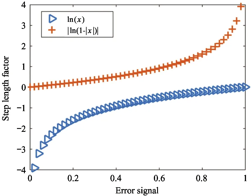
Fig.2 Basic logarithmic function curve

It can be seen from Fig.2 that the change rule of step size of ln(x) curve is contrary to what is needed. Further transform, replacexwith 1-x. In this case, ifxis the error signal, ln(x) is the step factor. When the error signal is large, the step factor also maintains a larger value to ensure the accelerated convergence of the algorithm; when the error signal is small, the step factor decreases, so that the algorithm has a small steady-state error. The purpose of taking absolute value ofxhere is to ensure that the value of ln(x) changes withxin accordance with the requirements. Here, in order to see the rule of image change more clearly, the image with absolute value of ln(x) is shown as the |ln(1-|x|)| curve in Fig.2.

It can be found that the change form of the |ln(1-|x|)| curve is in accordance with the rule that the step factor follows the change of the error signal. Next, the effect of introducing symbolic function on step size factor is discussed. The updated formula of currentρ(n) is as follows.

ρ(n)=(1-λ)e(n-1)sign(x(n-1))

+λ(n-1)

(38)

Second, by adding anti-jump factorβ, the step-size factor of the algorithm changes smoothly in the later period, to reduce the steady-state error. Therefore, the logarithmic function is introduced, which is Eq.(9).

When the absolute values of ln(1-|e(n)|) andβare 5.0, 4.0, 3.0, 2.0, 1.0 and 0.5 respectively, the change of step factor and error signal is shown in Fig.3.

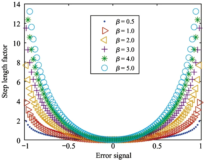
Fig.3 Function curves with variable parameters after introducing logarithmic and symbolic functions

From Fig.3, it can be found that the step size is adjusted by symbolic function and logarithmic function, and the step factor curve shows good convergence and stability. The step size factor is also associated with the input signal and the error signal, which enhances the anti-interference ability of the algorithm.

In order to verify the superiority of the improved algorithm further, the new algorithm is used in the experiment of active micro-vibration control.

4 Active micro vibration control experiments based on new algorithms

4.1 Construction of experimental platform

In this experiment, the 3 DOF active micro-vibration control unit is designed and fabricated to verify the control algorithm.

The active vibration isolation structure of three-degree-of-freedom micro-vibration is shown in Fig.4, which mainly includes base, vibration-starting module, vibration-suppressing module and loading platform. The base is mainly used to load and fix the whole isolation model structure. The starting module is used to simulate the micro-vibration response of the structure caused by external disturbances. The vibration suppression module can suppress the micro-vibration caused by the starting module through active vibration control. The vibration suppression module is fixed to the platform, and the vibration response of the platform is measured by capacitive displacement sensor.

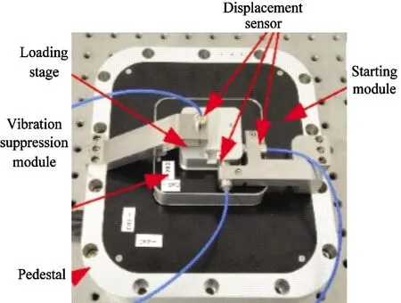
Fig.4 Pitcure of the 3 DOF active micro-vibration control unit

The 2 computers are connected by cross-network to construct xPC real-time system. Two NI-6289 data acquisition boards are inserted into the PCI slot of the target computer as AD input and DA output of the experimental system. Before the experiment, the C code generated by the control program on the host computer is downloaded to the target computer. In the experiment, the target machine outputs a disturbance signal of 0-10 V to the power amplifier (E00.D6, XMT©), which is amplified to 0-150 V. The excitation module simulates the external disturbance to generate the perturbation response.

On this basis, based on high performance computer, DA and AD card, signal conditioner, power amplifier related measurement and control instruments, and the development environment of Matlab/Simulink software, a multi-degree-of-freedom structural model active vibration isolation experimental system is constructed for experimental analysis and verification of structural active vibration control methods. The specific structure of the experimental system is shown in Fig.5.

Fig.5 Block diagram of the 3 DOF active micro-vibration control system

Displacement transducer (E509.C1, XMT©) collects vibration signal of the carrier platform, and after signal conditioner (E09.C1, XMT©) conditioning, it becomes 0-10 V voltage signal and enters the target machine for real-time processing. Through the operation of the controller in the target machine, the control signal of 0-10 V is output. After amplification of the power amplifier, the vibration suppression module is driven to act to suppress the micro-vibration of the platform. The experimental system of active vibration isolation for micro-vibration of three-degree-of-freedom model structure is shown in Fig.6.

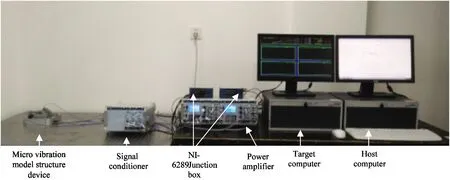
Fig.6 Experimental setup of the 3 DOF active micro-vibration control system

After the experimental platform is built, the performance of the new algorithm will be verified by the micro-vibration active control experiment.

4.2 Active control experiment of micro-vibration

For the convenience of experiment, thex-direction is chosen as the direction of the experiment. In this experiment, the sampling frequency is set to 1 000 Hz, the order of adaptive filter is set to 24, and the value of noise is set to 0. The total time of this experiment is 100 s. The time of applying disturbance signal at 0 s and suppressing signal is at 5 s respectively.

4.2.1 Convergence verification experiment

For comparison of algorithms, the parameters of each algorithm are adjusted experimentally, and the convergence speed of each algorithm is compared under the same steady-state error condition. Here, the sum of the steady-state errors of algorithms in the experiment from 95 s to 100 s is made. And the sum of the above-mentioned steady-state errors is recorded as errorsum. If the errorsum of each algorithm is equal, it is considered that each algorithm finally reaches the same steady state error. In the experiment, the values ofφandλare 1 020.988 and 0.97, respectively, and the lower limit factorδminis -465. From the comprehensive comparison of experiments, in addition to the above 4 algorithms, a fixed step size algorithm is added. For the comparison of the intuitive, experiment compare the micro vibration effect of the algorithm with the other 4 algorithms in the time, as shown in Fig.7.

As can be seen from Figs.7(a)-(d), the improved algorithm curve (the algorithm in this paper) and the other curves (the other 4 algorithms) almost coincide in the last 5 s of the experiment. Compared with the other 4 algorithms, the new algorithm reduces the steady-state error by 95% in the shortest time. That is, under the same degree of inhibition, the convergence speed of the improved algorithms curve is obviously faster than that of the other 4 algorithms.

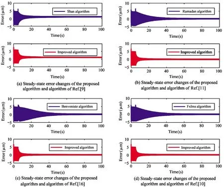
Fig.7 Comparison of steady-state errors between the proposed algorithm and other algorithms

To observe the overall convergence rate of each algorithm from the beginning of vibration suppression to the end of this process, the mean square error (MSE) of this algorithm and the 4 algorithms mentioned above are drawn in the graph. MSE is defined as

MSE(n)=E(e2(n))

(39)

where, MSE is the value of the mean of the square ofe(n). The MSE results of each algorithm are shown in Fig.8.

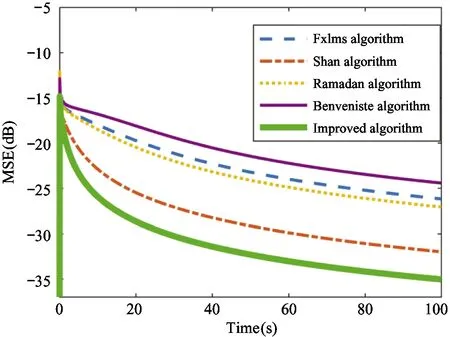
Fig.8 MSE curve of each algorithm

Under the same steady-state error, the MSE curves of each algorithm in Fig.8 can be seen. In the experimental process, improved algorithm in this paper not only has small steady-state error, but also has a faster convergence speed than the other 4 algorithms. The above results show that the convergence speed of improved algorithm has been greatly improved.

4.2.2 Steady-state error verification experiment

The next step is to verify the steady-state error of improved algorithm. The verification method is to let each algorithm run in the same time and get the steady-state error of each algorithm in the final time.

For the convenience of experiment, 3 000 sampling points with time interval of 5-8 s are selected in this paper. The steady-state error changes of each algorithm in the same time interval are shown in Fig.9.

Between 5 s and 8 s, Fig.9 shows that the new algorithm has a fast convergence speed in the experimental. And after 5.1 s, the convergence speed of improved algorithm is much smaller than the other 4 algorithms. By the end of 8 s, the steady-state error of this algorithm is also much smaller than that of other algorithms. It is concluded that, compared with other algorithms mentioned above, the proposed algorithm not only has fast convergence speed, but also has small steady-state error after convergence.

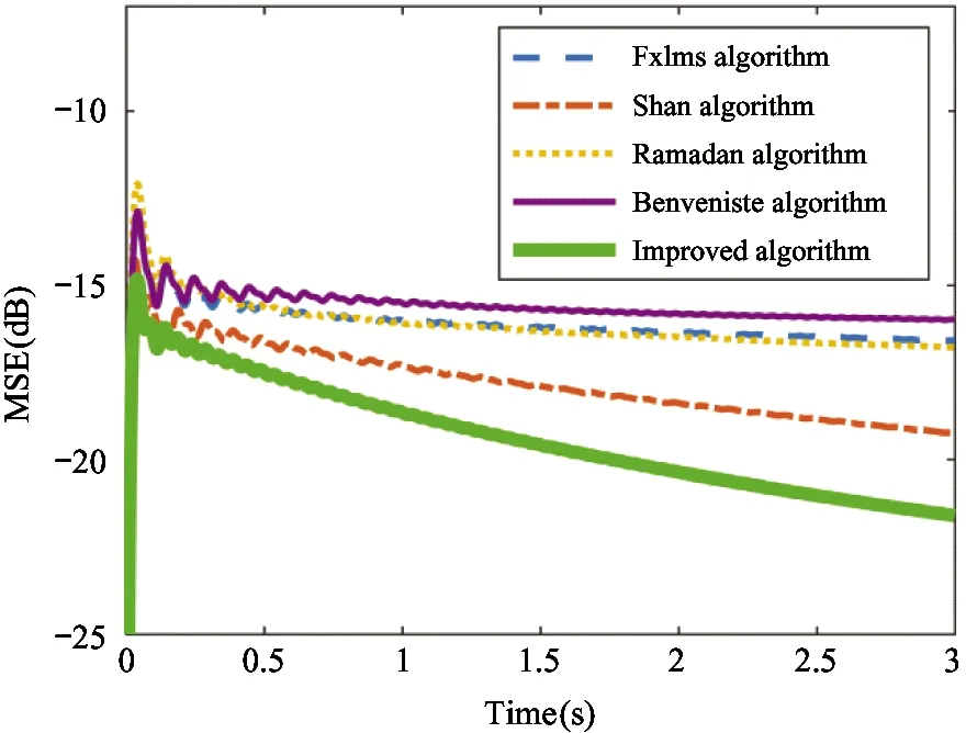
Fig.9 Steady-state error curve of each algorithm

In order to increase the comparative intuitiveness of experimental data of each algorithm, the vibration suppression rate and steady-state error results of each algorithm in the experiment of 20 s are taken to make Table 1. In order to compare the fairness of the experimental results, the sum of the steady-state errors in the last 5 s of the experiment is approximately the same.

Under the same steady-state error, the performance of each algorithm is analyzed by comparing the results of vibration suppression rate and steady-state error at 20 s. From Table 1, it can be seen that the maximum vibration suppression rate of the proposed algorithm is 91.48% at 20 s, which is much higher than that of the other 4 algorithms at this time, and the steady-state error of the proposed algorithm is also the minimum of 0.0341, which is much lower than that of the other 4 algorithms at this time.

Table 1 Data comparison of each algorithm

From the analysis of the above experimental data and charts, it can be seen that the proposed algorithm is applied to the experiment of active micro-vibration control, which verifies the superiority of the algorithm in convergence and steady-state error.

5 Conclusion

The traditional algorithm and the existing variable step size LMS algorithm are thoroughly analyzed, and then a new adaptive filtering algorithm based on input signal and error signal is proposed. In the proposed algorithm, logarithmic function and symbolic function are introduced to establish the updating method of step factor. When the steady-state error is large, the new step-size factor will be updated to a larger value to accelerate the convergence of the algorithm to the steady-state. On the contrary, when the steady-state error is small after the convergence, the step-size factor will keep a smaller value to reduce the steady-state error. Then the convergence and steady-state error of the new algorithm are deduced theoretically. After that, the influence of parameters on the step size factor is analyzed. And the performance of the existing variable step size algorithm is improved. Finally, in order to verify further the superiority of the algorithm, it is applied to the micro-vibration active control experiment. The experimental results show that the proposed algorithm is superior to other algorithms in convergence and steady-state error. It shows that the proposed algorithm has good performance and practical application value.