Method for predicting cuttings transport using artificial neural networks in foam drilling

PAK Kumdol, PENG Jianming, RI Jaemyong, CHOE Kumhyokand HO Yinchol

1. School of Resource Exploration Engineering, Kim Chaek University of Technology, Pyongyang 999093, D.P.R. Korea;2. College of Construction Engineering, Jilin University, Changchun 130026, China;3. School of Information Science and Technology, Kim Chaek University of Technology, Pyongyang 999093, D.P.R. Korea

Abstract: Foam is used widely in underbalanced drilling for oil and gas exploration to improve well perfor-mance. Accurate prediction of the cutting transport and pressure loss in the foam drilling is an important way to prevent stuck pipe, lost circulation and to increase the rate of penetration(ROP).In foam drilling, the cuttings transport quality may be defined in terms of cuttings consistency and downhole pressure loss, which are controlled by many factors. Therefore, it is very difficult to establish the mathematical equation that reflects nonlinear relationship among various factors. The field and experimental measurements of these parameters are time consuming and costly. In this study, the authors suggest a cuttings transport mathematical modeling using BPN (back propagation network), RBFN (radial basis function network) and GRNN (general regression neural network) based on various experiment data of cuttings transport of previous researchers and compared the result with experiment data. Results of this study show that the GRNN has a correlation coefficient of 0.999 62 and an average error of 0.15 in training datasets, and a correlation coefficient of 0.998 81 and an average error of 0.612 in testing datasets, which has higher accuracy and faster training velocity than the BP network or RBFN network. GRNN can be used in many mathematical problems for accurate estimation of cuttings consistency and downhole pressure loss instead of field and experimental measurements for hydraulic design in foam drilling operation.

Keywords: cuttings transport; underbalanced drilling; foam

0 Introduction

High-efficiency drilling is essential for the exploitation of oil and gas. Inefficient cuttings transport will cause many problems in the process of drilling including high torque, high drag, premature bit wear, and even stuck pipe (Heydari,etal., 2017; Rooki & Rakhshkhorshid, 2017; Akhshik & Rajabi, 2018; Pangetal., 2019).

During the drilling, when conventional drilling fluids are used, the hydrostatic pressure may be larger than the formation pressure and it may become the reason for lost circulation and serious damage in the reservoir, especially in low-pressure reservoir. Underbalanced drilling keeps the bottom-hole pressure (BHP) below the reservoir pressure which allows the leakage of oil and gas into well during drilling process, helping the cutting transport process.

Foam drilling is one of the underbalanced drilling methods for better drilling performance. Foam fluids generally consist of 5%--25% of liquid phase and 75%--95% of gaseous phase. The liquid phase could be fresh water or brines while the gaseous phase must be an inert gas, such as nitrogen, carbon dioxide and air. Surfactant accounts for about 5% of the liquid phase. Foam fluids help to improve the productivity of drilling process via increasing the rate of penetration (ROP), minimizing the formation damage, minimizing the lost circulation and avoiding the stuck pipe situations.

How to effectively remove cuttings with foam is critical to the drilling process. The cuttings with the foam could create problems similar to those with conventional drilling fluid, which may completely fail in controlling down-hole pressure.

Most studies of cuttings transport in foam drilling are experimental and in numerical modeling stage (Chenetal., 2007; Duanetal., 2010; Suradietal., 2015; Naderi & Khamehchi, 2018; Pangetal., 2019; Arild, 2014; Cayeuxetal., 2014).

Initially, the majority of researches related to cuttings transport with foam described operators’ experiences, field practices, and one-dimensional numerical simulations of the cuttings transport process. Experimental investigations were the major ways to observe cuttings transport and analyze the effects of different parameters on that with a gas-solid-liquid three-phase flow by using foam. Many researchers established large-scale simulated flow loops. In these investigations, a lot of experiments have been carried out for the rheological property of foam and regression model has been studied (Duan, 2007; Duanetal., 2010; Suradietal., 2015).

In foam drilling, the computation of cutting transportation process is much more complicated than a single-phase fluid case due to the characteristics of foam fluids. Therefore, it is very difficult to establish the mathematical equation that reflects nonlinear relationship among various factors. Also, the field and experimental measurements of these parameters are time consuming and costly.

Meanwhile, computational fluid dynamics (CFD) software like FLUENT is also applied to simulate the cuttings transport behavior with foam in various conditions, and it also provides some additional information that is difficult to obtain for experimental observations (Rookietal., 2014; Yanetal., 2014). Many mathematical models using artificial neural networks (ANNs), genetic algorithm(GA) and ant crowd algorithm(ACA) have been introduced in cuttings transport with foam. In recent years, ANNs have become very useful tools to develop models which express the interrelationship between the input and the output of complicated systems. Moreover, an attempt has been made to develop a neural network model to predict the cuttings concentration as a function of key output parameters in foam drilling (Rookietal., 2014, Rooki, 2015, Rooki & Rakhshkhorshid, 2017).

In foam drilling, the cuttings transport quality may be defined in terms of properties such as cuttings consistency and downhole pressure loss.

This paper aims to make simple and cost effective artificial neural networks (ANN) to establish the relationships between input data including foam velocity, foam quality, concentration of polymer, pressure, temperature, and pipe rotation and output data including cuttings concentration and pressure loss based on various experiment data of cuttings transport of previous researchers.

1 Forward neural network

In forward neural network, there are BPN (back propagation network), RBFN (radial basis function network), GRNN (general regression neural network) and so on. Forward neural network consists of input layer, hidden layer and output layer.

1.1 BPN

BPN has capability of interpolating and generalizing well. But it may require a considerable training time, and it is not sure if toy can get the best global solution. Each problem has its optimal number of hidden layers and nodes, and the optimum number depends on the problem itself and decides its accuracy. Unfortunately, there are many difficulties to determine the optimum number till now. Hence, we have to use trial and error procedure to develop a BPN.

1.2 RBFN

RBFN is an extremely powerful type of feed-forward ANN, which differs strongly from BPN in activation functions and how they are used. The RBFN has the approximation accuracy advantages over other commonly employed networks such as BPN. Furthermore, RBFN has the advantages of short training time, generality and simple network architecture. The ‘linear in the parameters’ property of RBFN guarantees the convergence of the parameters to the global minimum. Moreover, the local tenability of RBFN only affect part of the nodes by any given inputs, and only a portion of the model parameters may need to be adjusted, so our raw database can be extended conveniently. Like most feed-forward networks, RBFN has three layers, namely, an input layer, a hidden layer, and an output layer. Theoretically, given sufficient samples, RBFN can approximate any continuous nonlinear function to arbitrary accuracy. Thus, RBFN is considered for implementing the cuttings transport fitting. The radbas transfer function was shown in Fig.1 (Rooki & Rakhshkhorshid, 2017).

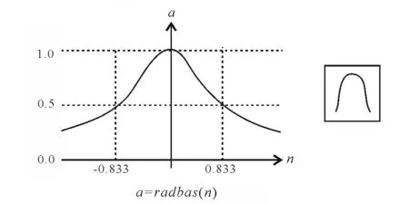
Fig.1 Radbas transfer function (Rooki & Rakhshkhorshid, 2017)

1.3 GRNN

GRNN is theoretically using the Parzen window estimator and was first applied as a neural network by Specht. GRNN is a variant of RBFN. It resembles to a normalized RBFN in which there is a hidden unit centered at every training case. These RBF units called kernels are usually probability density function such as the Gaussian. Given a sufficient number of hidden neurons, GRNN can approximate a continuous function to an arbitrary accuracy.

IfX(vector with dimensionp) andy(scalar) are random variables, andXandyare measured values, we definef(X,y) as the joint continuous probability density function. Iff(X,y) is known, it is easy to estimate the expected value ofyas:

(1)

The advantage of GRNN over other regression schemes, however, is thatf(X,y) need not be known. Specht showed that the joint probability density function can be estimated from observation as:

(2)

WhereXiandyiare the observed samples of inputs and outputs that constitute the training set,nis the number of sample observations andpis the dimension of the vector variableX. Substituting (2) in (1) yields

(3)

(4)

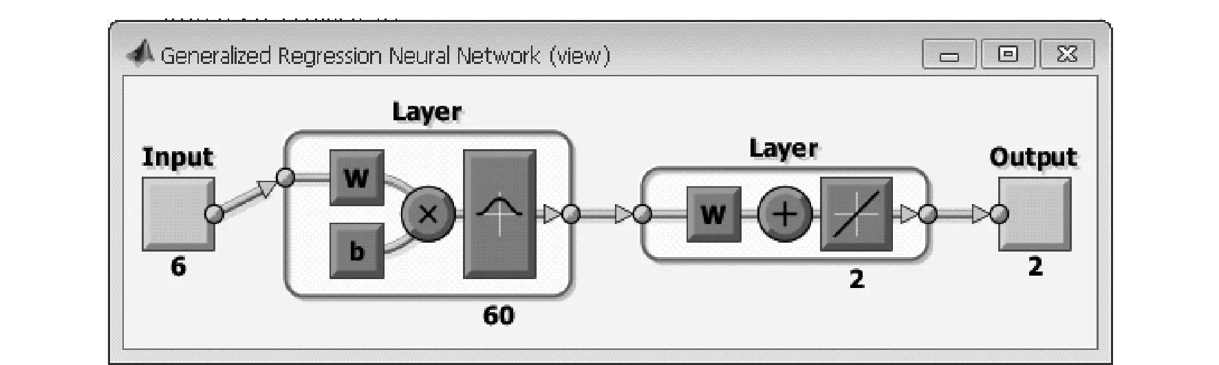
Fig.2 Structure of GRNN in Matlab

At a node in the second layer the exponential values for all samples are summed, while at the other nodes the product of the exponent value and the corresponding observed outputyifor each sample observation is calculated. At the node in the third layer all the product values are added up, which is then supplied to the output node, where the ratio of the sum of the exponent and the product values is calculated. Compared to the back-propagation method, the weighting coefficients between the layers depend upon the observedXi,yi, and the smoothing parameterσ. Instead of training the weighing coefficients repeatedly, only a suitable single value ofσis needed to predict the output. Therefore, the GRNN is able to represent the characteristics in a much shorter time than back-propagation method.

GRNN also can be designed in MATLAB software. The code automatically chooses the number of training patterns as the number of the hidden layer neurons.

The mean relative error (MRE) and the correlation coefficient (R) were used for evaluation of ANN efficiency.

(5)

(6)

2 Cuttings concentration and pressure loss estimation using ANN

In this study, the experimental data (70 data samples) of cuttings transport using foam from literature (Duan, 2007; Chenetal., 2007) were used for ANN modeling.

For training and testing ANN, 60 of 70 experimental datasets were selected for training and the rest 10 datasets were selected for testing purposes.

The ANN was trained by different spread constant (SPREAD) for GRNN and RBFN to achieve the optimum SPREAD according toMREandRbetween experimental and predicted value in training and testing data. Meanwhile, BPN model was constructed for comparing analysis.

As can be seen, it is composed of three layers as follows:

(1) Input layer: the neurons of the input layer are effective parameters (6 inputsP,T,V,RPM, Г,C) in this study.

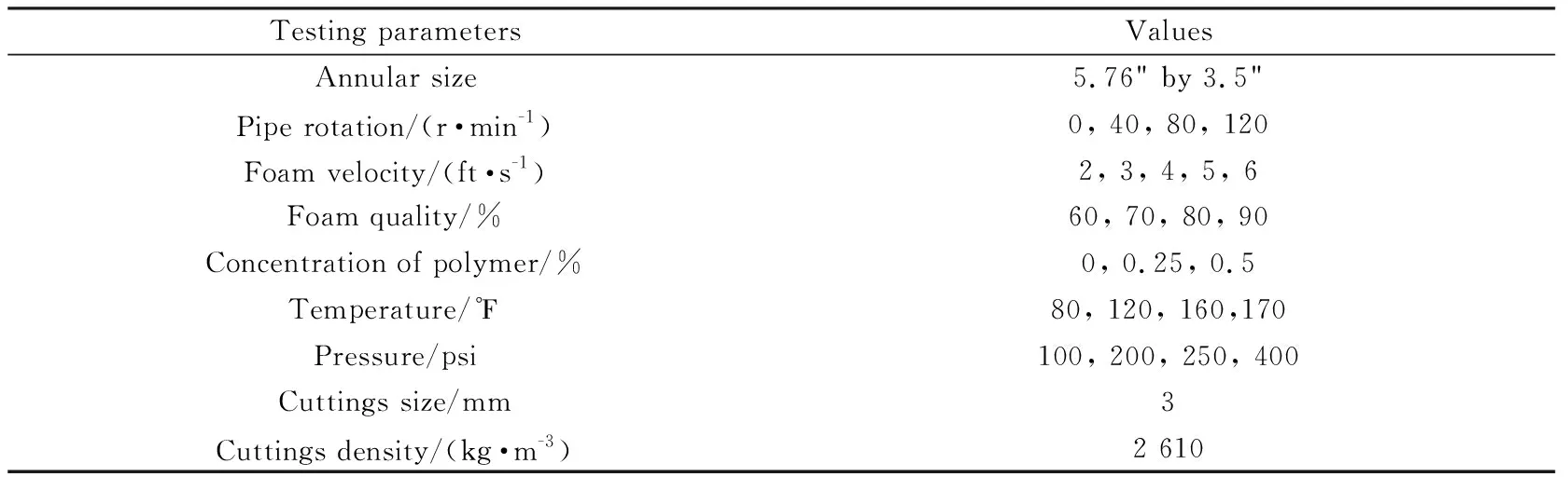
Table 1 Test matrix of cuttings transport using aqueous foam (Duan, 2007; Chenet al., 2007)

(2) Hidden layer: In RBFN and GRNN, the number of the neurons in the hidden layer can be simply considered equal to the number of training patterns in all neurons. Furthermore, in the designing process of RBFN and GRNN, a proper spread value to control the sensitivity of hidden neurons needs to be determined. In this work,MSEwas used to find the proper value of SPREAD. After some trial and error, the va-lues of SPREAD of RBFN and GRNN were set equal to 0.67 and 0.1, respectably. In BPN, the number of hidden layers was 10.

3 Results and discussion

The BPN, RBFN and GRNN codes were designed in MATLAB software. 60 of 70 data samples from the literature were used to train the ANN for the estimation of cuttings concentration and pressure loss in annulus from input variables (V,C,P,T,RPM, Г). 10 samples were used for testing ANN.

Fig.3a shows comparison result of the predicted value and the measured data for the training data in GRNN.

The correlation coefficient (R) is 0.999 62 with theMREvalue of 0.15, describing the appropriate training of GRNN. To ensure correct training, the network was tested using the test data. Fig.3b illustrates the results of GRNN for the testing data versus experimental data. The correlation coefficient (R) is 0.998 81 with theMREvalue of 0.612, describing the appropriate testing of GRNN. Also, results of RBFN for training and testing process are the same as GRNN.

Fig.3 Comparison results of predicted value and measured data for training data (a) and testing data (b) in GRNN

Results of BPN show a correlation coefficient of 0.982 96 and an average error of 6.75 for training datasets, and a correlation coefficient of 0.960 34 and an average error of 19.87 in testing datasets.

Table 2 shows the operational parameters, experimental and prediction data of ANN in testing data. The results of GRNN and RBFN are compared with results of BPN in Table 3.

The result shows that both RBFN and GRNN have good convergence and high accuracy above BPN and can model the process of cuttings transport with accuracy. So RBFN and GRNN can be used for hydraulic design in drilling operation, instead of field and experimental measurement. However, the training time of RBFN and GRNN is different; the training time of GRNN is 3 times faster than that of RBFN.

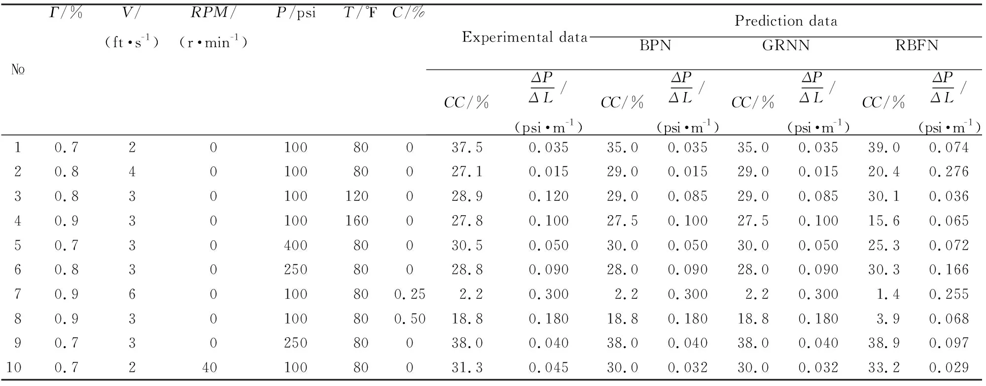
Table 2 Operational parameters, experimental and prediction data of ANN in test data

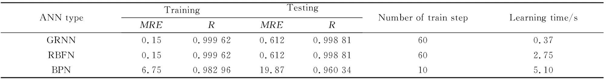
Table 3 Fitting errors of GRNN, RBFN and BPN

4 Conclusion

In this paper the ANN model with three layers was applied for estimating cuttings concentration and pressure loss in foam drilling from effective parameters (foam velocity, foam quality, concentration of polymer, pressure, temperature, and pipe rotation). Three ANNs, namely, BPN, RBFN and GRNN have been trained and compared under the same conditions. Hidden layer has 60 neurons. Two criteria (RandMRE) were used for various ANN evaluations. AnMREof 0.15 and a correlation coefficient of 0.999 62 (in the training phase), and anMREof 0.612 and a correlation coefficient of 0.998 81 (in the testing phase) indicate the advantages of the GRNN and RBFN model such as faster training, high accuracy and simple structure.

GRNN and RBFN exhibited satisfying fitting abi-lity. It showed that GRNN and RBFN have the advantages of simple architecture, good precision and short computational time. According to the comparisons on the training results, it is shown that the RBFN and GRNN are more effective than the BPN, So RBFN and GRNN can be used in many mathematical problems such as this study instead of BPNN and CFD modeling.