A Finite-difference Approximation for the Oneand Two-Dimensional Tempered Fractional Laplacian

Yaoqiang Yan · Weihua Deng · Daxin Nie

Abstract This paper provides a f inite-difference discretization for the one- and two-dimensional tempered fractional Laplacian and solves the tempered fractional Poisson equation with homogeneous Dirichlet boundary conditions. The main ideas are to, respectively, use linear and quadratic interpolations to approximate the singularity and non-singularity of the one-dimensional tempered fractional Laplacian and bilinear and biquadratic interpolations to the two-dimensional tempered fractional Laplacian. Then, we give the truncation errors and prove the convergence. Numerical experiments verify the convergence rates of the order O (h2-2s).

Keywords Tempered fractional Laplacian · Finite-difference scheme · Linear and quadratic interpolations · Bilinear and biquadratic interpolations · Convergence rates

1 Introduction

Fractional Laplacian is a nonlocal (anomalous) diff usion operator, which describes the motion of the particles with inf inite propagation speed and divergent second moments of the jump length. The study of nonlocal (anomalous) diff usion [ 7] is of great signif icance in many applications, such as the f inance [ 5, 11], the electric current [ 10], and the porous media f low [ 9]. In the research of the stochastic process theory, the fractional Laplacian is the generator of the Lévy process [ 3]. At present, there are some valuable articles discussing the fractional Laplacian in mathematical theories and numerical methods. For example,[ 1] introduced the f inite-element approximation for the n-dimensional fractional Laplacian with the homogeneous Dirichlet boundary condition, [ 2] presented the code employed for implementation in two-dimensional cases, and [ 8] proposed a f inite-difference discretization using the weighted trapezoidal rule to approximate the fractional Laplacian and proved the convergence in one dimension.

To well describe the particles with the f inite propagation speed, the tempered fractional Laplacian is proposed in [ 6]. This paper focuses on solving the tempered fractional Poisson equation with the homogeneous Dirichlet boundary condition, that is

where the tempered fractional Laplacian is def ined as

with

and the domain is taken as Ω≜Ωn=[-1,1]n, n=1,2 . Our main ideas of designing the numerical schemes are to use the linear and quadratic interpolations and the bilinear and biquadratic interpolations to, respectively, approximate the non-singular and singular parts of ( 2) in the one- and two-dimensional cases, and utilize the fact that the obtained coeff icient matrix is a symmetric positive def inite Toeplitz matrix to reduce the computational complexity.

This paper is organized as follows. Section 2 gives the discretization for ( 2) and the f inite-difference scheme of Eq. ( 1) in one dimension, and then, we prove the truncation error and convergence. Section 3 provides the numerical scheme in two dimensions, whose organization is similar to Sect. 2. In the last section, several numerical experiments are carried out to verify the orders of convergence.Finally, we introduce the inner products and norms used in this paper. The inner product and norm of discrete l2are

The norm of discrete l∞and continuous L∞are

2 One-Dimensional Case

In this section, we discuss the f inite-difference scheme and the convergence of Eq. ( 1) in the one-dimensional case.

2.1 Numerical Scheme

In the one-dimensional case, we f irst divide Ω1into -1=x-N＜…＜x0＜…＜xN=1 with xi=ih , h=1∕N . For i=-N+1,-N+2,…,N , we have

where D1=[-2,2] . In the following, we denote

We use the linear interpolation to approximate the non-singular part of ( 3) in[kh,(k+1)h] , that is

The quadratic interpolation is applied to approximate the singular part of ( 3) in [-h,h] , that is

Combining ( 3), ( 4), and ( 5), we have

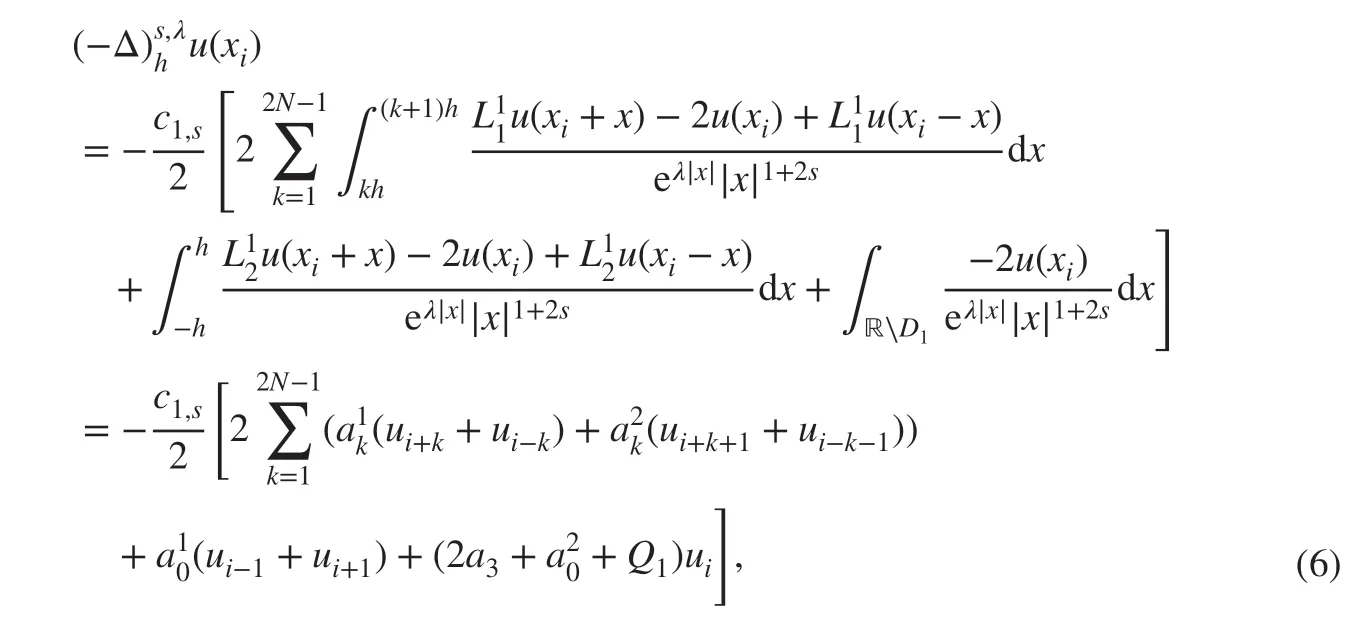
where ui=u(ih) and

where

The matrix form of ( 8) is

where

2.2 Truncation Error

Theorem 2.1Let u(x)∈C3(ℝ) with the compact support [-1,1] andbe the discretization of (-Δ)s,λ. Then,

where C is a constant independent of h.

ProofFor xi∈Ω1, from ( 6), we have

For the f irst part of ( 13), there exists

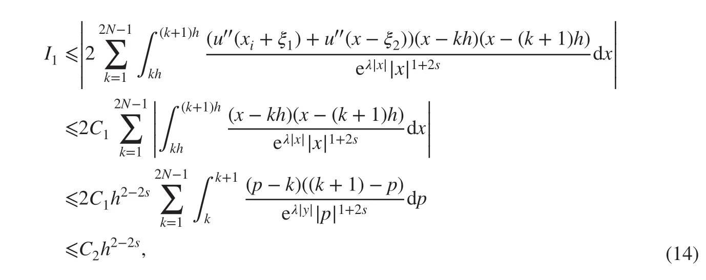
According to ( 5) and ( 15), there exists

which implies I2≤Ch3-2s. Combining ( 13), ( 14), and ( 16) results in ( 12).

2.3 Convergence

In this subsection, we prove the convergence of Eq. ( 10). First, we provide the property of the matrix B1def ined in ( 11).

Theorem 2.2The matrix B1is strictly diagonally dominant, that is

ProofAccording to ( 6), ( 8), and ( 9), we have

and

Combining ( 7) completes the proof.

From Theorem 2.2 and ( 11), it can be noticed that all the eigenvalues of the coeff icient matrix B1are positive, implying that B1is a symmetric positive def inite matrix.

Theorem 2.3Suppose u( x) is the exact solution of Eq. ( 1), and uhis the solution of the f inite-difference scheme ( 10). Then,

where C is a constant independent of h.

ProofDenoting Eh=u-uh, taking the inner product of Ehon B1Eh, and by the Cauchy-Schwarz inequality, we have

where λmin(B1) is the minimal eigenvalue of B1. Then,

From Theorem 2.1, we have

Supposing ‖Eh‖∞=, according to ( 6) and Q1＜0 , we have

which implies

From Theorem 2.1, we have

3 Two-Dimensional Case

In the section, we discuss the f inite-difference discretization and convergence for Eq. ( 1) in the two-dimensional case.

3.1 Numerical Scheme

In the two-dimensional case, we divide Ω2=[-1,1]2into Ξhevenly with h=1∕N , and-1=x-N＜…＜x0＜…＜xN=1 , -1=y-N＜…＜y0＜…＜yN=1 . For i,j=-N+1,-N+2,…,N-1 , there exists

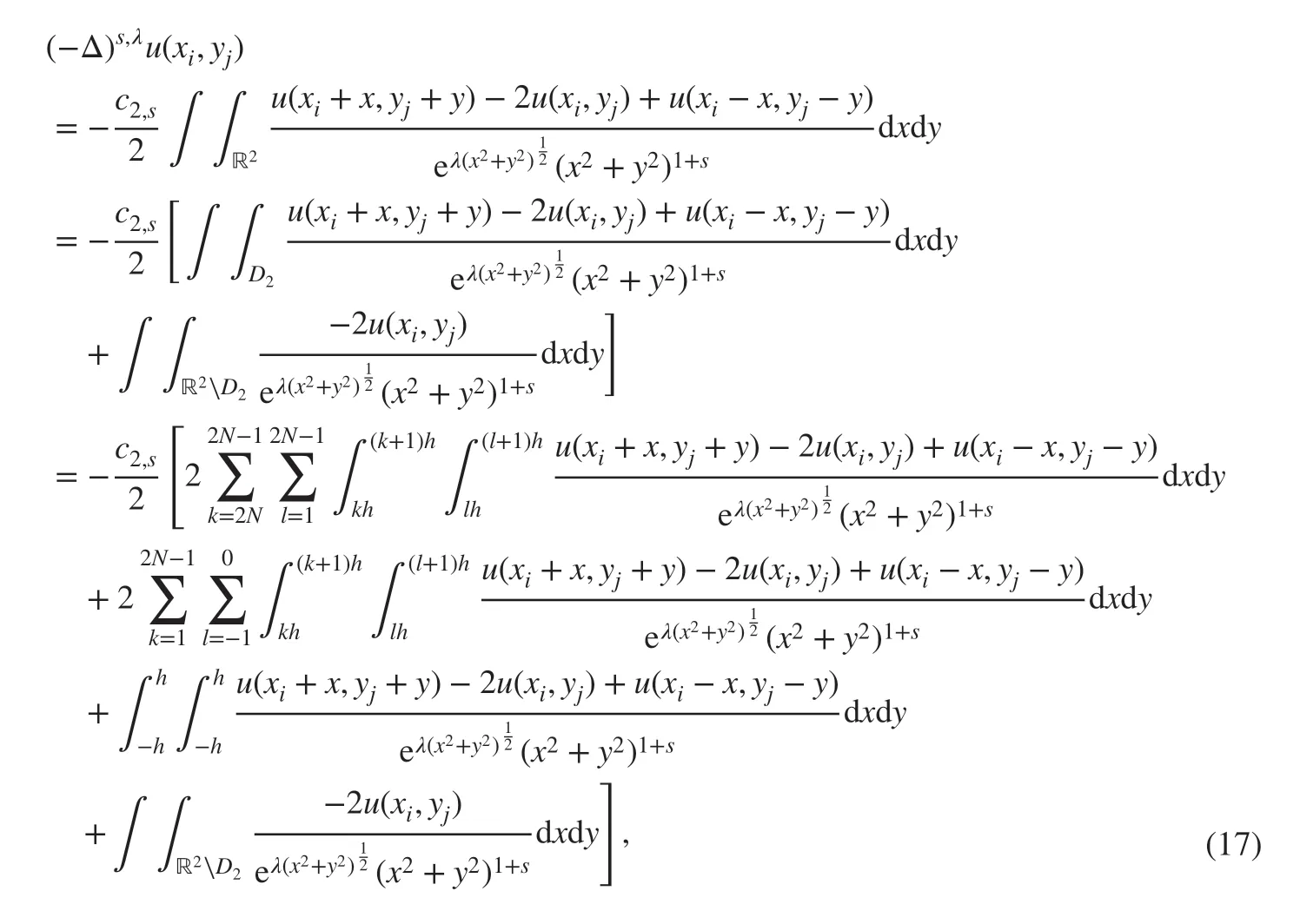
where D2=[-2,2]2. In addition, we setdxdy.

To approximate the non-singular part of ( 17) using the bilinear interpolation on[kh,(k+1)h]×[lh,(l+1)h] , we have

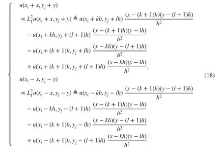
For the singular part of ( 17), using biquadratic interpolation on [-h,h]×[-h,h] leads to

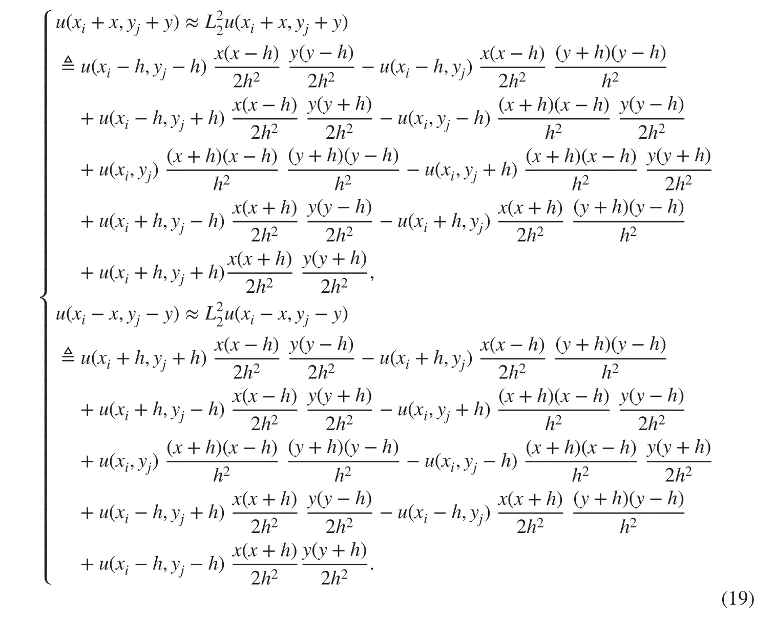
By ( 18) and ( 19), there exists

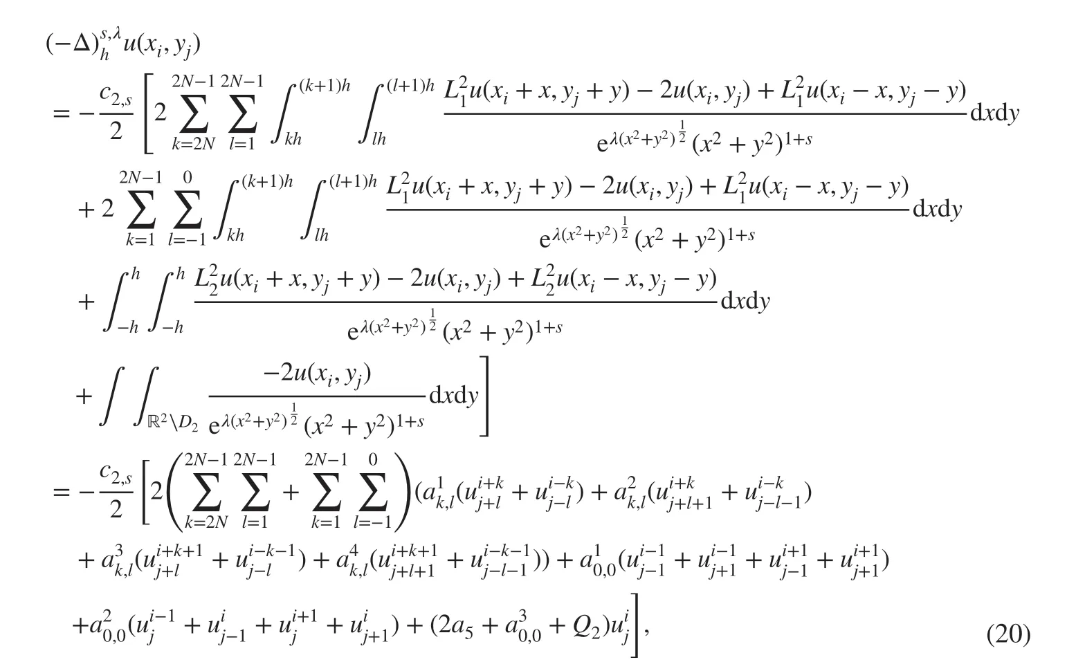
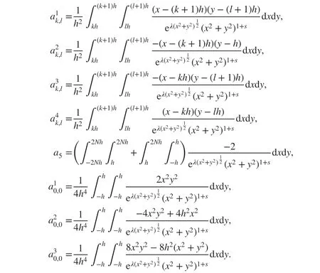
Then, we get the discretization scheme

where

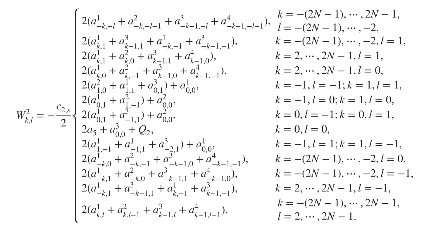
The matrix form of ( 21) can be written as

where

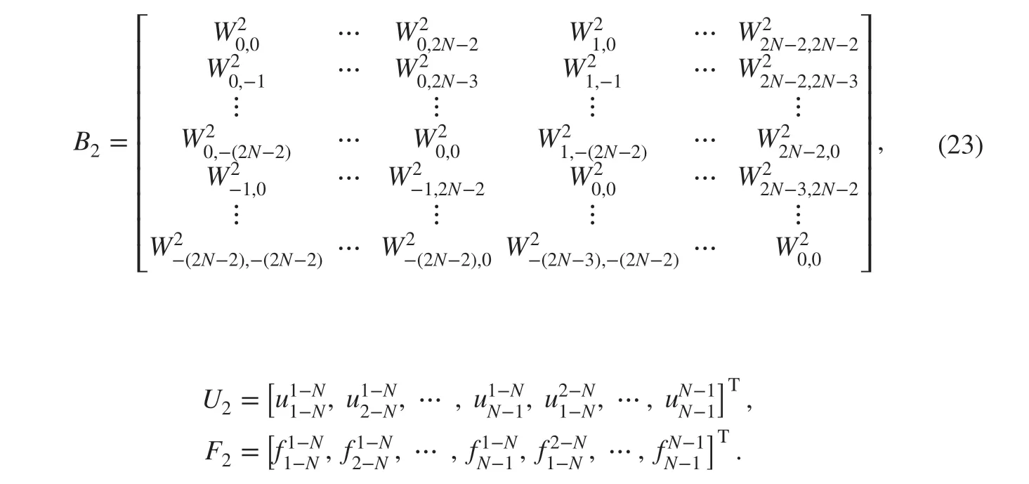
Remark 3.1The matrix B2is made up of block of Topelitz from ( 23). To reduce the computational cost, one can use CG or PCG by [ 5] in numerical experiments, and the memory requirement is O(N2) and the computational cost is O(N2logN2) instead of O(N4) and O(N6).

3.2 Truncation Error

Lemma 3.1[ 4] Let I denote the bilinear interpolation on the box K=[0,h]×[0,h]. For f∈W2,∞(K) ( Wk,p(K) denotes the Sobolev space), the error of the bilinear interpolation is bounded by

Theorem 3.1Let u(x,y)∈C3(ℝ2) with the support Ω2⊂ℝ2anddenote an approximation of (-Δ)s,λin ( 21). Then,

where C is a constant independent of h.

ProofFor (xi,yj)∈Ξh, according to ( 17) and ( 20), we have

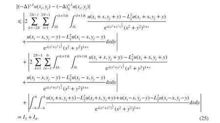
Denoting the f irst two parts of ( 25) as I3, using Lemma 3.1, we have

Denoting the last part of ( 25) as I4, from

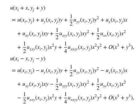
we have

According to ( 19), there exists

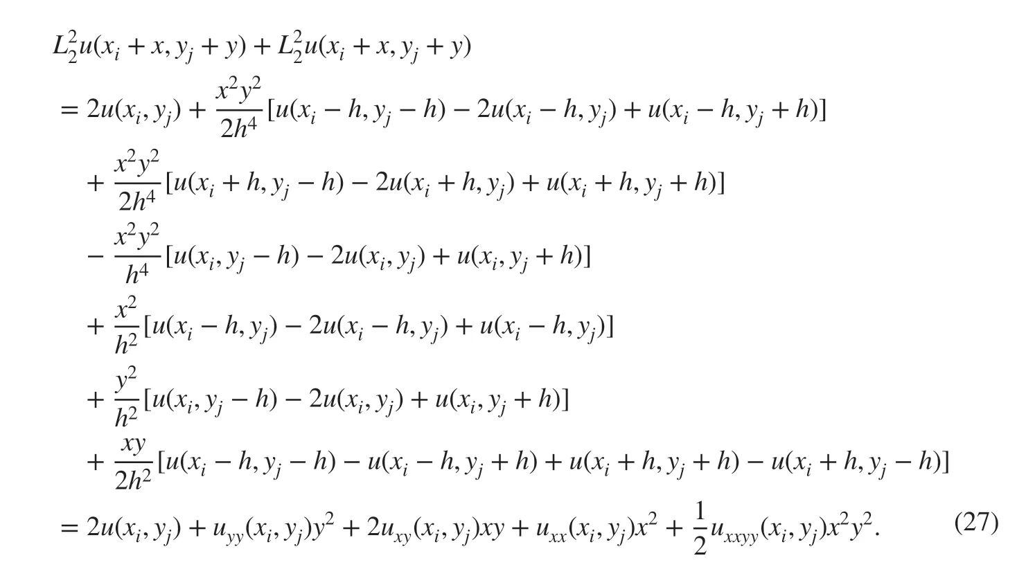
From ( 26) and ( 27), |I4|≤Ch3-2scan be obtained.

3.3 Convergence

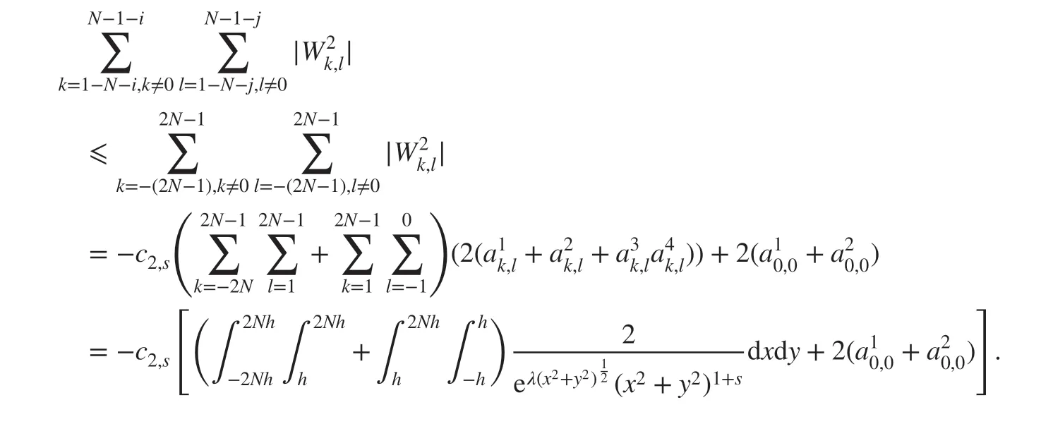
Theorem 3.2The matrix B2is strictly diagonally dominant in ( 23), that is

ProofCombining ( 20) and ( 21) leads to

According to the fact

and Theorem 3.2, the proof is completed.

Theorem 3.3Suppose that u( x, y) is the exact solution of Eq. ( 1), and uhis the solution of the f inite-difference scheme ( 22). Then,

where C is a constant independent of h.

ProofThe proof is similar to Theorem 2.3.

4 Numerical Experiments

This section performs the numerical experiments to verify the orders of convergence, which validate the eff ectiveness of our algorithm. In the numerical experiments, especially in the implementation of two-dimensional cases, f( x, y) needs to be numerically calculated. For(xi,yj)∈Ξh, u(x+xi,y+yj) is supported on [-1-xi,1-xi]×[-1-yj,1-yj], and u(x-xi,y-yj) is supported on [-1+xi,1+xi]×[-1+yj,1+yj].

According to the symmetry of the operators, we just need to calculate it in the f irst quadrant(Fig. 1). Then,

Fig. 1 Integral region of (xi,yj) in the f irst quadrant

where

The last part of ( 28) is

Example 1Consider u(x)=(1-x2)2as the exact solution of Eq. ( 1) in one dimension and u(x,y)=(1-x2)2(1-y2)2in two dimensions, and λ=0.5 . One can see that the convergence rate is O(h2-2s) in Tables 1 and 2.

Table 1 Errors and convergence rates when λ=0.5 in one dimension

Table 2 Errors and convergence rates when λ=0.5 in two dimensions

Example 2We take λ=0 , and the solution is similar to Example 1. Tables 3 and 4 show that the convergence rate is O(h2-2s).

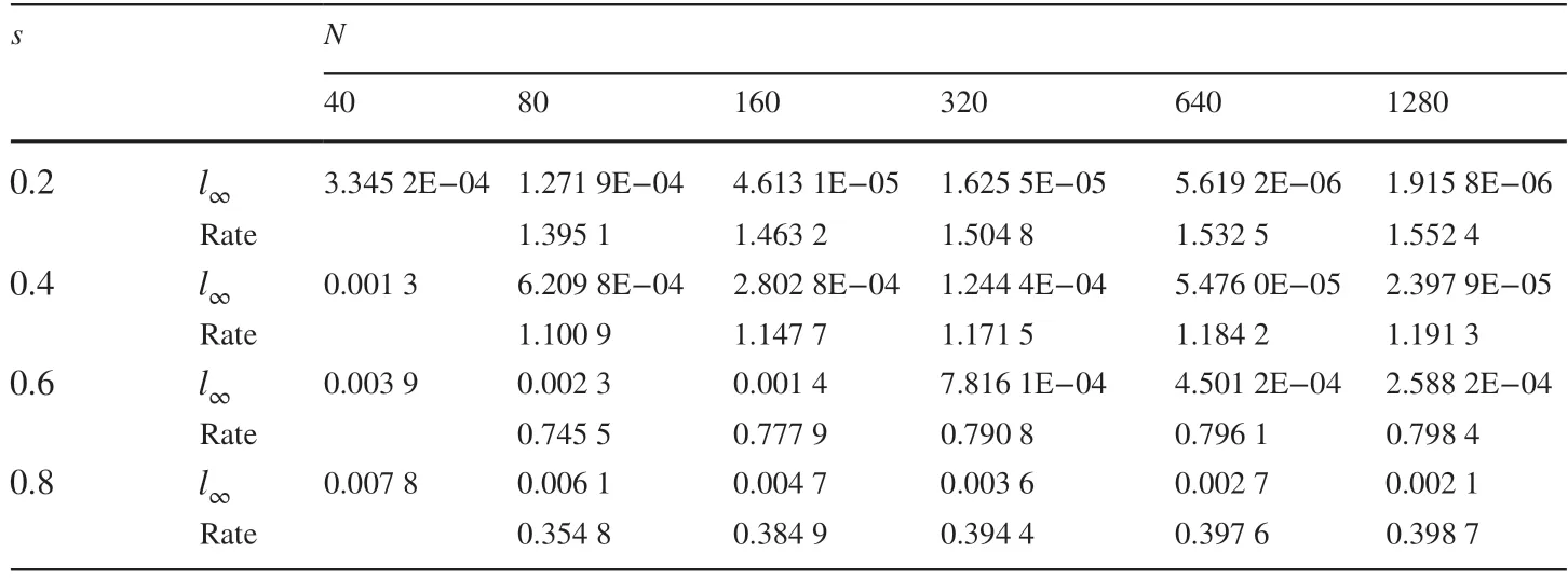
Table 3 Errors and convergence rates when λ=0 in one dimension

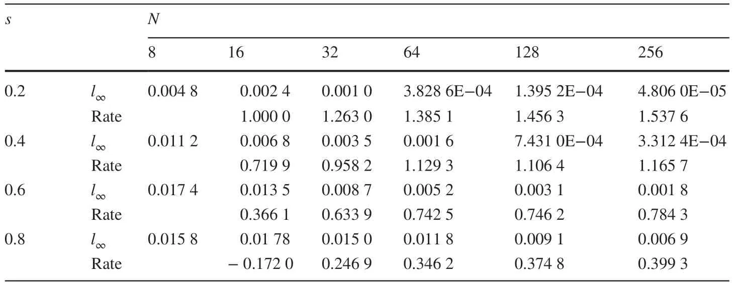
Table 4 Errors and convergence rates when λ=0 in two dimensions

5 Conclusion

This paper provides the f inite-difference schemes for the tempered fractional Poisson equation with homogeneous Dirichlet boundary conditions in one and two dimension cases. From Theorems 2.3 and 3.3, one can notice that the convergence rate is O(h2-2s) ,being conf irmed by the numerical experiments.

AcknowledgementsThis work was supported by the National Natural Science Foundation of China under Grant No. 11671182 and the Fundamental Research Funds for the Central Universities under Grant No.lzujbky-2018-ot03.