Numerical Algorithm for the Time-Caputo and Space-Riesz Fractional Diff usion Equation

Yuxin Zhang · Hengfei Ding

Abstract In this paper, we develop a novel f inite-difference scheme for the time-Caputo and space-Riesz fractional diff usion equation with convergence order O (τ2-α+h2) . The stability and convergence of the scheme are analyzed by mathematical induction. Moreover, some numerical results are provided to verify the eff ectiveness of the developed difference scheme.

Keywords Caputo derivative · Riesz derivative · Fractional diff usion equation

1 Introduction

With the development of science, it has been found that the fractional derivatives and fractional differential equations provide an excellent instrument for the description of memory and hereditary properties of various materials and processes. Therefore, they are widely used in the f ield of science and technology, such as the f ields of control theory, biology,electrochemical processes, porous media, viscoelastic materials [ 7, 14, 15].

However, unfortunately, for most fractional differential equations, it is not an easy task to seek for their analytical solutions. For some simple linear equations, even if the analytic solutions are obtained, it is not convenient to calculate, because the analytic solutions contain some special functions. Therefore, it is essential to develop the eff ective numerical solutions of the fractional differential equations.

Since the numerical approximation of fractional derivatives is the most important step in numerical solutions of fractional differential equations, we f irst review the progress made in numerical approximation of fractional derivatives. As for the Caputo derivative, Gao et al. proposed a so-called L1-2 formula with order ( 3-α) [ 8]. Using the diff erent methods, Li et al. also got a numerical differential formula with convergence order ( 3-α) [ 11]. Later, Alikhanov proposed another ( 3-α) th order numerical differential formula at the superconvergence point t =tj+σ, and named it as the L2-1 formula [ 1]. Furthermore, Li et al. developed a series of high-order formulas using the r th ( r≥4 is a positive integer) degree interpolation function [ 9]. For approximating the Riesz fractional derivative, the f irst-order accurate normal/shifted Grünwald formula [ 13], second-order accurate weighted and shifted Grünwald by choosing the appropriate weight coeffi cients [ 16], second-order accurate fractional centered difference formula [ 3], and some other higher-order formulas [ 5, 6, 20] have been constructed. Based on the above mentioned and other approximation formulas, a tremendous amount of f inite-difference methods for solving the fractional differential equations have been developed. For example, Cui constructed a compact f inite-difference scheme with the temporal accuracy of f irst order and spatial accuracy of fourth order for the one-dimensional fractional diff usion equation in [ 2]. Wang and Vong [ 17]developed two high-order f inite-difference schemes for the fractional modif ied anomalous subdiff usion equation and the diff usion-wave equation, respectively. Based on the fractional multistep methods in time and central difference formula in space, Zeng [ 19]proposed several f inite-difference schemes for solving the time-fractional diff usionwave equation.

In this paper, we propose a novel f inite-difference scheme for the following time-Caputo and space-Riesz fractional diff usion equation:

This paper is organized as follows. In Sect. 2, based on a second-order accuracy approximation operator for the Riesz fractional derivative, we develop a f inite-difference scheme for the time-Caputo and space-Riesz fractional diff usion equation. The stability and convergence analysis of the constructed scheme is studied in Sect. 3. Numerical results are provided in Sect. 4 to demonstrate the eff ectiveness of the numerical algorithm.

2 The Development of the Numerical Algorithm

First, we introduce the following L 1 formula [ 10, 14] to numerical treatment of the Caputo fractional derivativeu(t) at t=tn(n=0,1,…,N):

where the weights are def ined by

and which have the following properties.

Lemma 1[ 12] Let bk=(k+1)1-α-k1-α,k=0,1,2,… and 0＜α＜1 . Then, one has

In [ 4], the authors constructed the following second-order numerical differential formula:

for the Riesz space fractional derivative, where the operators

and

Here, the coeffi cients

can be obtain by the novel generating function

Besides, we can also calculate the coeffi cientsby the following recursive relations:

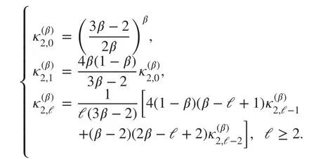
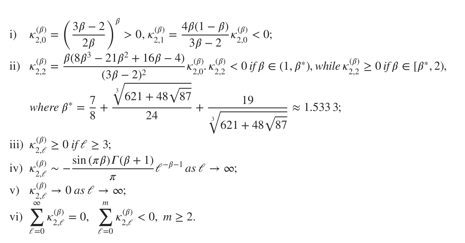
Next, we list the properties of the coeffi cientsℓ=0,1,…).

Lemma 2[ 4] The coeffi cients(ℓ=0,1,…) have the following properties for 1＜β＜2:

Now, we consider Eq. ( 1) at point (xj,tk) . For the space fractional derivative, we apply the second-order formula ( 3) to approximate the Riesz derivative for x∈(0,L) , that is,

where

and

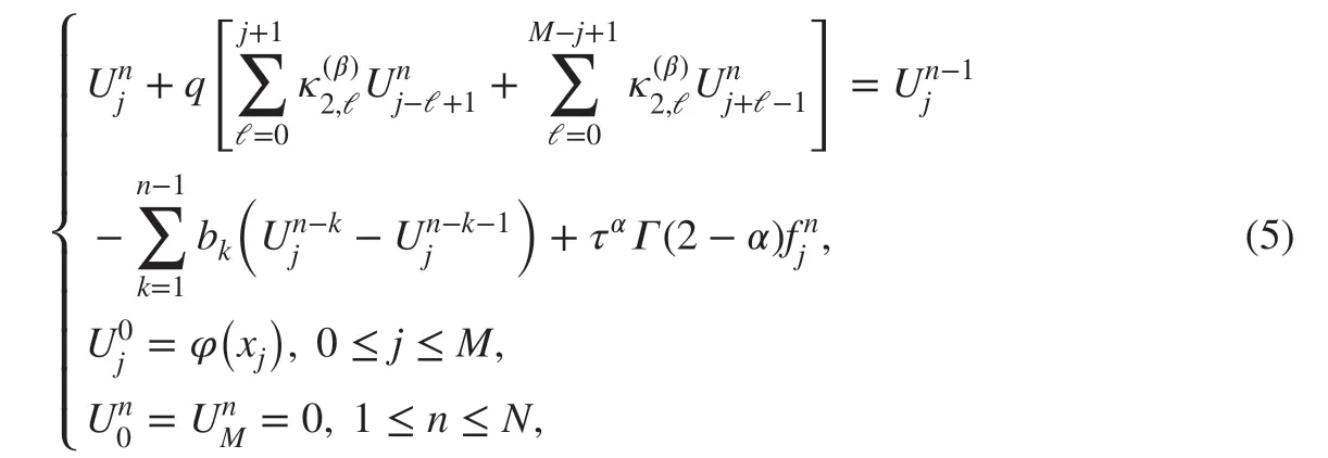
Finally, substituting ( 2) and ( 4) into ( 1), and omitting the high-order terms O(τ2-α+h2) .Replacing the function u(xj,tn) with its numerical approximation value, we can obtain the following f inite-difference scheme:

3 Stability and Convergence Analysis

In this section, the stability and convergence analysis of the above difference scheme are studied in detail.

3.1 Stability Analysis

From Lemma 2, we easily know that

Lemma 3Under the condition the coeffi cientsatisfy

Theorem 1Under the condition ( 6) and 0＜α＜1 , the f inite-difference scheme for the time-Caputo and space-Riesz fractional diff usion equation ( 1) is unconditionally stable.

ProofLetbe the exact solution of the f inite-difference scheme ( 5). Denote, then we can obtain the following perturbation equation:

Below, we will discuss the stability of the numerical algorithm by mathematical induction.Denote

Furthermore, let

and assuming that we have proved that ‖‖Ek‖‖∞≤‖‖E0‖‖∞for 1≤k≤n-1. Then, we also know that

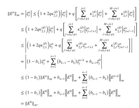
This ends the proof.

3.2 Convergence Analysis

Theorem 2Denote by u(xj,tn)(j=1,2,…,M-1;n=1,2,…,N) the exact solution of ( 1)at mesh point (xi,tn) , and let {|0≤j≤M,0≤n≤N} be the solution of the f inite-difference scheme ( 5). Def ine

then there exists a positive constant C, such that

under the condition ( 6) and 0＜α＜1.

ProofDenote. then it follows from ( 1) and ( 5) that

Below, we give the convergence result using mathematical induction. First, for the case of n=1 , let

Then, one has

Using ε0=0 andthen there holds that

As the before, set

and

then we further have

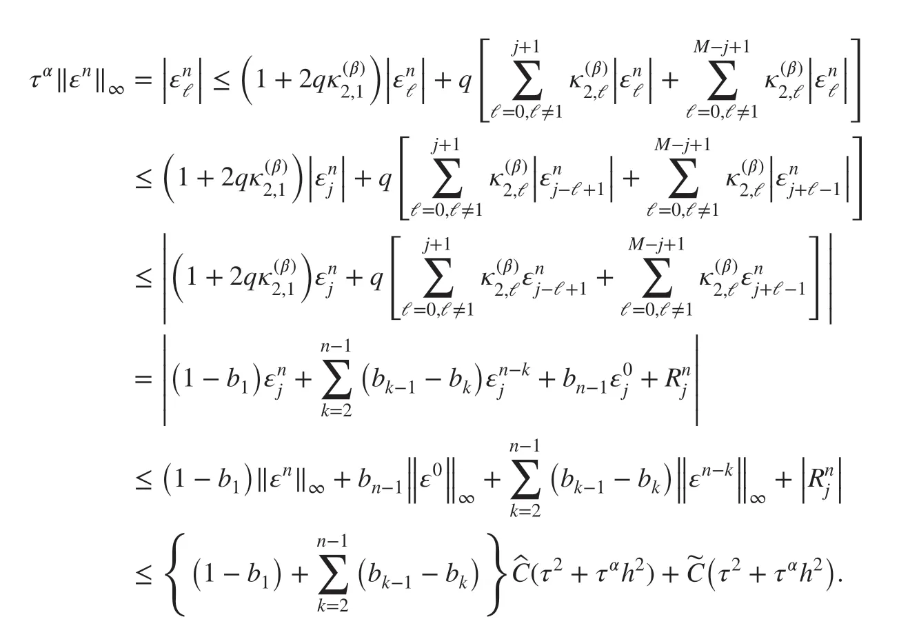
Therefore, there exists a positive constant C, such that

This f inishes the proof.

4 Numerical Examples

In this section, we apply the method proposed in this paper to solve the fractional partial differential equation. We obtain the numerical results and plot graphs for these problems with the help of MATLAB routines.

Example 1Let us consider the following equation:

on a f inite domain 0≤x≤1,0≤t≤1 with a given force term

Its analytical solution is

Tables 1 and 2 list the maximum errors and convergence orders using the f inite-difference scheme ( 5) at time t=1 with diff erent stepsizes. It is observed that the numerical convergence orders are consistent with our theoretical analysis. In addition, Figs. 1,2, 3 and 4 compare the graphs of the exact and approximate solutions with diff erent values of α , β , τ , and h. The graphs show excellent agrement between the solutions.

Table 1 Temporal convergence ordersofExample 1 with β =1.6 and h=

Table 1 Temporal convergence ordersofExample 1 with β =1.6 and h=

α τ The maximum errors The temporal convergence orders 0.2 1 10 3.100 519E-005 -1 15 1.573 542E-005 1.672 7 1 20 9.722 013E-006 1.673 8 1 25 6.700 211E-006 1.668 2 1 30 4.951 918E-006 1.658 4 0.4 1 10 1.245 707E-004 -1 15 6.713 991E-005 1.524 4 1 20 4.318 225E-005 1.534 2 1 25 3.063 135E-005 1.538 9 1 30 2.312 765E-005 1.541 2 0.6 1 10 3.782 137E-004 -1 15 2.189 031E-004 1.348 6 1 20 1.480 504E-004 1.359 4 1 25 1.091 674E-004 1.365 4 1 30 8.505 257E-005 1.369 1 0.8 1 10 1.010 018E-003 -1 15 6.309 231E-004 1.160 5 1 20 4.504 827E-004 1.171 0 1 25 3.464 536E-004 1.176 7 1 30 2.793 741E-004 1.180 3

Table 2 Spatial convergence orders of Example 1 with α=0.4 and τ=

Table 2 Spatial convergence orders of Example 1 with α=0.4 and τ=

β h The maximum errors The spatial convergence orders 1.6 1 10 2.155 992E-003 -1 15 9.409 768E-004 2.044 8 1 20 5.276 218E-004 2.011 0 1 25 3.335 257E-004 2.055 4 1 30 2.303 227E-004 2.030 7 1.7 1 10 2.208 103E-003 -1 15 9.633 981E-004 2.045 6 1 20 5.397 315E-004 2.014 0 1 25 3.413 537E-004 2.053 2 1 30 2.357 280E-004 2.030 7 1.8 1 10 2.230 580E-003 -1 15 9.751 993E-004 2.040 6 1 20 5.467 731E-004 2.011 3 1 25 3.464 373E-004 2.045 0 1 30 2.394 909E-004 2.024 9 1.9 1 10 2.217 223E-003 -1 15 9.740 071E-004 2.028 8 1 20 5.476 063E-004 2.001 7 1 25 3.481 438E-004 2.029 8 1 30 2.412 347E-004 2.012 1

Fig. 1 Comparison of exact and numerical solutions for Example 1 with τ= t=0.5,h= at time

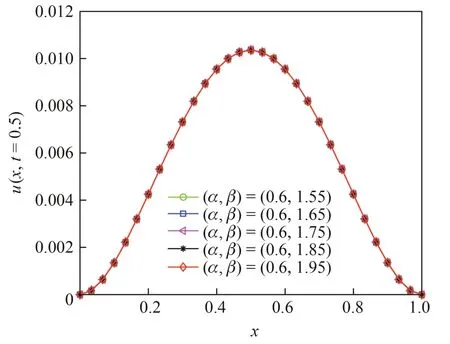
Fig. 2 Comparison of exact and numerical solutions for Example 1 with τ= t=0.5,h= at time

Fig. 3 Comparison of exact and numerical solutions for Example 1 with τ= x=0.8,h=at space

Example 2Consider the following equation:

where

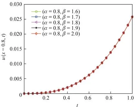
Fig. 4 Comparison of exact and numerical solutions for Example 1 with τ= x=0.8,h=at space

The exact solution is

In Table 3, we list the maximum error for β=1.2,h=1∕500 and diff erent values of α . In Table 4, we list the maximum error for α=0.7,τ=1∕400 and diff erent values of β .From these tables, we can conclude that the developed numerical solutions are in excellent agreement with the exact solution.

Table 3 Temporal convergence orders of Example 2 with β=1.2 and h=

Table 3 Temporal convergence orders of Example 2 with β=1.2 and h=

α τ The maximum errors The temporal convergence orders 0.15 1 10 5.992 925E-006 -1 15 3.119 961E-006 1.609 9 1 20 1.961 602E-006 1.613 1 1 25 1.372 343E-006 1.601 0 1 30 1.028 883E-006 1.579 9 0.35 1 10 2.032 757E-005 -1 15 1.102 994E-005 1.507 8 1 20 7.106 417E-006 1.528 1 1 25 5.043 203E-006 1.536 9 1 30 3.808 692E-006 1.539 9 0.55 1 10 5.827 195E-005 -1 15 3.382 003E-005 1.341 8 1 20 2.284 980E-005 1.363 0 1 25 1.681 387E-005 1.374 6 1 30 1.306 956E-005 1.381 7 0.75 1 10 1.300 527E-004 -1 15 8.070 317E-005 1.176 8 1 20 5.724 104E-005 1.194 1 1 25 4.375 770E-005 1.203 7 1 30 3.509 557E-005 1.209 9 0.95 1 10 2.682 839E-004 -1 15 1.781 985E-004 1.009 1 1 20 1.328 735E-004 1.020 2 1 25 1.056 765E-004 1.026 3 1 30 8.758 086E-005 1.030 2

Table 4 Spatial convergence orders of Example 2 with α=0.7 and τ=

Table 4 Spatial convergence orders of Example 2 with α=0.7 and τ=

β h The maximum errors The spatial convergence orders 1.55 1 10 1.625 279E-004 -1 12 1.142 747E-004 1.932 0 1 14 8.480 268E-005 1.935 0 1 16 6.548 636E-005 1.935 8 1 18 5.214 072E-005 1.934 9 1.65 1 10 1.548 145E-004 -1 12 1.084 935E-004 1.950 1 1 14 8.032 008E-005 1.950 5 1 16 6.190 909E-005 1.949 7 1 18 4.921 736E-005 1.947 8 1.75 1 10 1.426 306E-004 -1 12 9.974 747E-005 1.961 5 1 14 7.372 765E-005 1.960 8 1 16 5.675 414E-005 1.959 5 1 18 4.507 008E-005 1.957 1 1.85 1 10 1.261 905E-004 -1 12 8.820 379E-005 1.964 3 1 14 6.515 927E-005 1.964 4 1 16 5.013 117E-005 1.963 5 1 18 3.979 032E-005 1.961 4 1.95 1 10 1.056 483E-004 -1 12 7.398 705E-005 1.953 8 1 14 5.471 822E-005 1.957 1 1 16 4.212 694E-005 1.958 4 1 18 3.345 178E-005 1.957 7

AcknowledgementsThe work was partially supported by the National Natural Science Foundation of China(no. 11561060).