ODE Methods in Non-Local Equations

Weiwei Ao,Hardy Chan,Azahara DelaTorre,Marco A.Fontelos,Mar´ıa del Mar Gonz´alezand Juncheng Wei

1 DepartmentofMathematicsandStatistics,WuhanUniversity,Wuhan430072,China;

2 Department of Mathematics,ETH Z¨urich,R¨amistrasse 101,8092 Z¨urich,Switzerland;

3 Dpto.de An´alisis Matem´atico.Facultad de Ciencias. Campus de Fuentenueva S/N.Universidad de Granada. 18071 Granada,Spain;

4 ICMAT,Campus de Cantoblanco,UAM,28049 Madrid,Spain;

5 Departamento de Matem´aticas,Universidad Aut´onoma de Madrid,UAM and ICMAT.Campus de Cantoblanco. 28049 Madrid,Spain;

6 Department of Mathematics,University of British Columbia,Vancouver,BC,V6T 1Z2,Canada.

Abstract. Non-local equations cannot be treated using classical ODE theorems. Nevertheless, several new methods have been introduced in the non-local gluing scheme of our previous article;we survey and improve those,and present new applications as well. First,from the explicit symbol of the conformal fractional Laplacian,a variation of constants formula is obtained for fractional Hardy operators. We thus develop, in addition to a suitable extension in the spirit of Caffarelli–Silvestre,an equivalent formulation as an infinite system of second order constant coefficient ODEs. Classical ODE quantities like the Hamiltonian and Wro´nskian may then be utilized.As applications, we obtain a Frobenius theorem and establish new Pohoˇzaev identities. We also give a detailed proof for the non-degeneracy of the fast-decay singular solution of the fractional Lane–Emden equation.

Key words: ODE methods,non-local equations,fractional Hardy operators,Frobenius theorem.

1 Introduction

Let γ∈(0,1). We consider radially symmetric solutions the fractional Laplacian equation

with an isolated singularity at the origin. Here

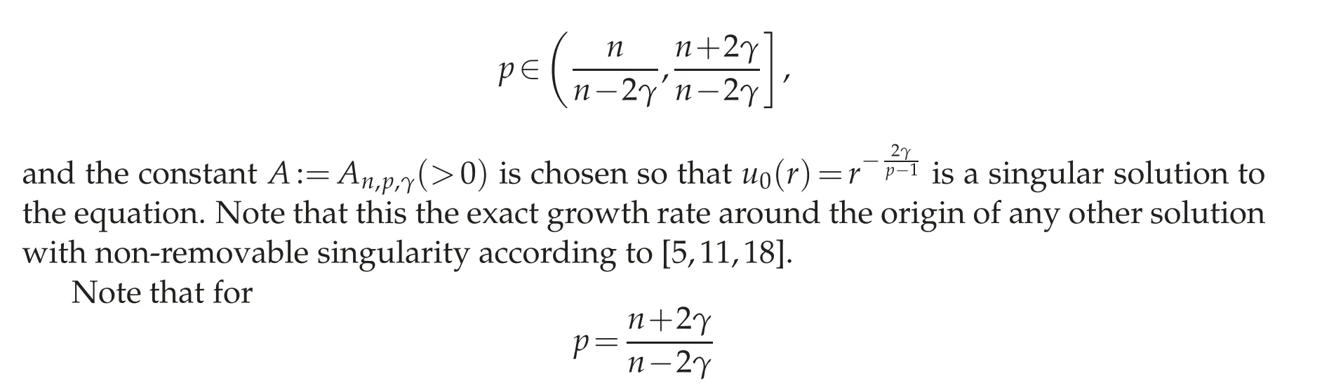
the problem is critical for the Sobolev embedding Wγ,2L2nn−2γ. In addition, for this choice of nonlinearity, the equation has good conformal properties and, indeed,in conformal geometry it is known as the fractional Yamabe problem. In this case the constant A coincides with the Hardy constant Λn,γgiven in(1.7).

There is an extensive literature on the fractional Yamabe problem by now. See[35,36,40,44]for the smooth case,[3,7,22,23]in the presence of isolated singularities,and[4,5,34]when the singularities are not isolated but a higher dimensional set.

In this paper we take the analytical point of view and study several non-local ODE that are related to problem(1.1),presenting both survey and new results,in the hope that this paper serves as a guide for non-local ODE. A non-local equation such as (1.1) for radially symmetric solutions u=u(r), r=|x|, requires different techniques than regular ODE. For instance, existence and uniqueness theorems are not available in general, so one cannot reduce it to the study of a phase portrait. Moreover,the asymptotic behavior as r→0 or r→∞is not clear either.

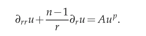
However,we will show that,in some sense,(1.1)behaves closely to its local counterpart(the case γ=1),which is given by the second order ODE

In particular,for the survey part we will extract many results for non-local ODEs from the long paper[5] but without many of the technicalities. However,from the time since[5]first appeared,some of the proofs have been simplified;we present those in detail.

The main underlying idea, which was not fully exploited in [5], is to write problem(1.1) as an infinite dimensional ODE system. Each equation in the system is a standard second order ODE, the non-locality appears in the coupling of the right hand sides(see Corollary 4.2). The advantage of this formulation comes from the fact that,even though we started with a non-local ODE,we can still use a number of the standard results,as long as one takes care of this coupling. For instance,we will be able to write the indicial roots for the system and a Wro´nskian-type quantity which will be useful in the uniqueness proofs. Other applications include novel Pohoˇzaev-type identities. We also hope that this paper serves as a complement to the elliptic theory of differential edge operators from[45,46]. Further use could include more general semi-linear equations such as the one in[16],but this is yet to be explored.

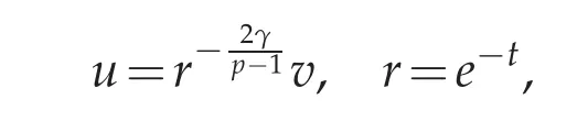
Let us summarize our results. First,in Section 3,we consider existence theorems for(1.1),both in the critical and subcritical case. We show that the change of variable

transforms(1.1)into the non-local equation of the form

for some singular kernel satisfying(t)～|t|−1−2γas|t|→0. The advantage of(1.3)over the original (1.1) is that in the new variables the problem becomes autonomous in some sense. Thus,even if we cannot plot it,one expects some kind of phase-portrait. Indeed,we show the existence of a monotone quantity(a Hamiltonian)similar to those of[9,10,29]which,in the particular case p=is conserved along the t-flow.

The proofs have its origin in conformal geometry and, in particular, we give an interpretation of the change of variable(1.2)in terms of the conformal fractional Laplacian on the cylinder. We also provide an extension problem for(1.3) in the spirit of the well known extension for the fractional Laplacian([12,49]and many others). Note,however,that our particular extension has its origins in scattering theory on conformally compact Einstein manifolds(see[14,17,37] and the survey[33],for instance)and it does not produce fractional powers of operators,but their conformal versions. This is the content of Section 2.

In addition,for p subcritical,this is,

we will also consider radial solutions to the linearized problem around a certain solution u∗. The resulting equation may be written as

Defining the radially symmetric potential V∗(r):=pAr2γup−1∗,this equation is equivalent to

Note that

for the positive constant

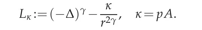
Therefore to understand operators with critical Hardy potentials such as L∗we will need to consider first the constant coefficient operator

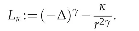
The fractional Hardy inequality ([8,30,39,41,42,50]) asserts the non-negativity of such operator up to κ=Λn,γ,hence whenever and this distinguishes the stable/unstable cases(see Definition 3.1).

Nonlinear Schr¨odinger equations with fractional Laplacian have received a lot of attention recently (see, for instance,[2,21,25]), while ground state solutions for non-local problems have been considered in the papers[28,29].

However, mapping properties for a linear operator such as L∗from (1.4), or even Lκ, had been mostly open until the publication of [5]. See also the related paper [31],which deals with mapping properties of powers of this operator in homogeneous Sobolev spaces,together with some applications from[32],where they prove the Scott conjecture for large atoms taking into account relativistic effects near the nucleus.

One of the cornerstones in[5]is to write a Green’s function for the constant coefficient operator Lκin suitable weighted spaces.While invertibility for Lκin terms of the behavior of its right hand side had been considered in [1], here we go further and calculate the indicial roots of the problem to characterize invertibility precisely.This is done by writing a variation of constants formula to produce solutions to Lκφ=h from elements in the kernel Lκφ=0. In particular, such φ is governed by the indicial roots of the equation.However, in contrast to the local case where a second order ODE only has two indicial roots, here we find an infinite number of them and, moreover, the solution is not just a combination of two linearly independent solutions of the homogeneous problem,but an infinite sum. We summarize those results in Section 4. We also present, in full detail,simplified proofs of the original statements.

One obtains, as a consequence, a Frobenious type theorem which yields a precise asymptotic expansion for solutions to(1.4)in terms of the asymptotics of the potential as r →0. Indeed, recall that we have that (1.5), so we can use what we know about Lκin order to obtain information about L∗. In particular, we find the indicial roots of L∗both as r→0 and as r→∞.

Next,we move on to original research. Section 5 is a combination of new and known results. There we give full account of non-degeneracy of Eq. (1.1) for the particular solution u∗,this is,we provide a characterization of the kernel of the linearized operator L∗,both in the stable and in the unstable cases.

One of the main contributions of this paper is the introduction of a new Wro´nskian quantity(5.6)for a non-local ODE such as(1.4),that allows to compare any two solutions,and plays the role of the usual Wro´nskian W=w′1w2−w1w′2for a second order linear ODE.While this quantity is close in spirit to that of[9,10,29], ours seems to adapt better to an autonomous non-local ODE.

Using similar techniques for the non-linear problem,we also provide new Pohoˇzaev identities: Proposition 6.1 (for the extension problem) and Proposition 6.2 (for the nonlocal problem formulated as a coupled ODE system).The underlying idea is that,switching from the radial variable r to the logarithmic t variable, and from the standard fractional Laplacian(−∆)γto the conformal fractional Laplacian Pγ,we are able to find conserved quantities since the resulting ODE is,though non-local,autonomous.

Some comments about notation:

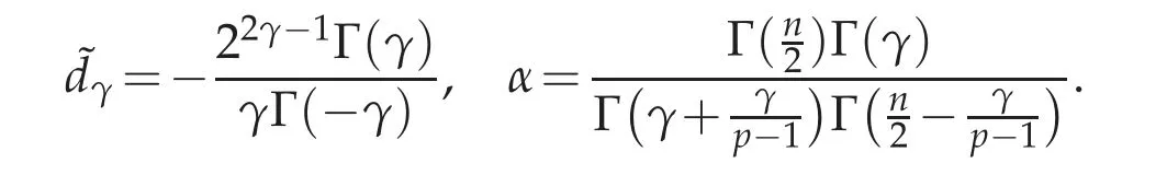
• The Hardy constant is given by

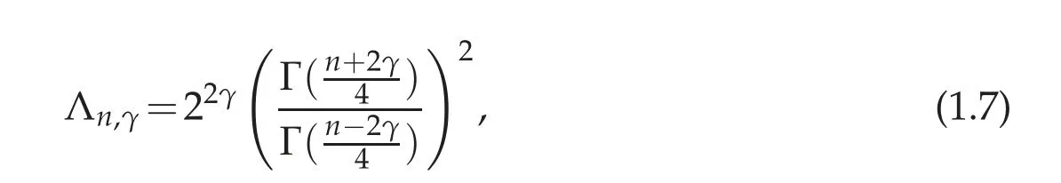
where Γ is the ordinary Gamma function.

• We write f1≍f2if the two (positive) functions satisfy C−1f1≤f2≤C f1for some positive constant C.

• While functions that live on Rnare represented by lowercase letters, their corresponding extension towill be denoted by the same letter in capitals.

• Snis the unit sphere with its canonical metric.

•2F1is the standard hypergeometric function.

2 The conformal fractional Laplacian on the cylinder

Most of the results here can be found in[5]. We review the construction of the fractional Laplacian on the cylinder R×Sn−1, both by Fourier methods and by constructing an extension problem to one more dimension.

2.1 Conjugation

Let us look first at the critical power,and consider the equation

It is well known[11]that non-removable singularities must be,as r→0,of the form

for a bounded function w.

We use conformal geometry to rewrite the fractional Laplacian operator(−∆)γon Rnin radial coordinates r>0,θ∈Sn−1. The Euclidean metric in polar coordinates is given by|dx|2=dr2+r2dθ2,where we denote dθ2for the metric on the standard sphere Sn−1. Now set the new variable

and consider the cylinder M=R×Sn−1,with the metric given by

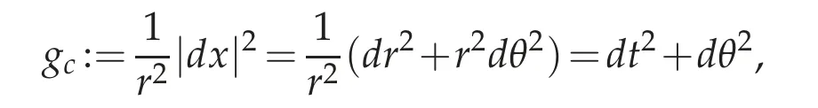
which is conformal to the original Euclidean one.

The conformal fractional Laplacian on the cylinder,denoted by Pγ,is defined in[22].We will not present the full construction here, just mention that its conformal property implies

and thus,if we define w by(2.2),in the new variables w=w(t,θ),then the original equation(2.1)transforms into

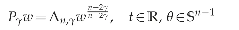
for a smooth solution w. Therefore we have shifted the singularity from the solution to the metric.

On the contrary,equation(1.1)for a subcritical power

does not have good conformal properties.Still,given u∈C∞(Rn{0}),we can consider

and define the conjugate operator

where we have defined the constant

The advantage of working withis that problem(1.1)is equivalent to

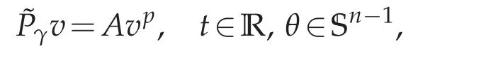
for some v=v(t,θ)smooth.

2.2 The operator as a singular integral

2.3 The extension problem

For γ ∈(0,1), this operator can also be understood as the Dirichlet-to-Neumann operator for an extension problem in the spirit of [12,14,17]. Before we do that, we need to introduce some notation.Define

Take the metric on the extension manifold Xn+1=(0,2)×R×Sn−1with coordinates R∈(0,2),t∈R,θ ∈Sn−1with standard hyperbolic metric

Note that the apparent singularity at R=2 has the same behavior as the origin in polar coordinates. This fact will be implicitly assumed in the following exposition without further mention.

The boundary of Xn+1(actually, its conformal infinity) is given by {R=0}, and it coincides precisely the cylinder Mn=R×Sn−1,with its canonical metric gc=dt2+dθ2.

Now we make the change of variables from the coordinate R to

The function ρ is known as the special(or adapted)defining function. It is strictly monotone with respect to R,which implies that we can write R=R(ρ)even if we do not have a precise formula and,in particular,ρ∈(0,ρ0)for

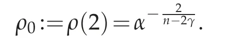
Moreover,it has the asymptotic expansion near the conformal infinity

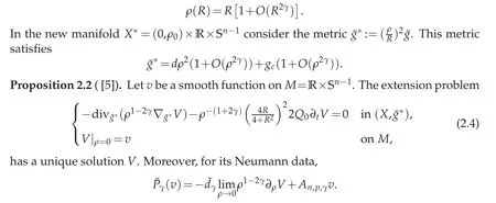
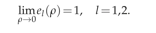
Remark 2.1([22]). If v is a radial function on M,this is,v=v(t),then the first equation in(2.4)decouples to

for some F(ρ)≥0 and some continuous functions el(ρ) which are smooth for ρ ∈(0,ρ0)and that satisfy

For convenience of the reader,let us particularize this result for Q0=0 in order to give a characterization for Pγw if w=w(t):

Proposition 2.3 ([22]). Let w=w(t) be a smooth, radially symmetric function on M=R×Sn−1. The extension problem

has a unique solution W=W(ρ,t). Moreover,for its Neumann data,

3 Non-local ODE:existence and Hamiltonian identities

In the following, we fix γ ∈(0,1). We consider radially symmetric solutions u=u(r) to the non-linear problem

3.1 The critical case

For this part,set

Let u=u(r)be a radially symmetric solution to

and set

then from the results in Section 2,we know that this problem is equivalent to

The advantage of the t variable over the original r is that one can show the existence of a Hamiltonian similar to the monotone quantities from[9,29]. However,in our case,it is conserved along the t-flow:

Theorem 3.1([5]). Let w=w(t)be a solution to(3.2)and set W its extension from Proposition 2.3. Then,the Hamiltonian quantity

The fact that such a Hamiltonian quantity exists suggests that a non-local ODE should have a similar behavior as in the local second-order case, where one can draw a phase portrait. However,one cannot use standard ODE theory to prove existence and uniqueness of solutions.

In any case,we have two types of solutions to(3.2)in addition to the constant solution w≡1:first we find an explicit homoclinic,corresponding to the standard bubble

Indeed:

Proposition 3.1([22]). The positive function

is a smooth solution to(3.2).

Second, we have periodic solutions (these are known as Delaunay solutions). The proof is variational and we refer to[23]for further details:

Theorem 3.2([23]). Let n>2+2γ.There exists L0(the minimal period)such that for any L>L0,there exists a periodic solution wL=wL(t)to(3.2)satisfying wL(t+L)=wL(t).

3.2 The subcritical problem

Now we consider the subcritical problem

Let u=u(r)be a radially symmetric solution to

and set

then(3.4)is equivalent to

for some v=v(t),t∈R.

Theorem 3.3 ([5]). Let v=v(t) be a solution to(3.5) and set V its extension from Proposition 2.2. Then,the Hamiltonian quantity Hγ[V](t)given in(3.3)is non-increasing in t.

The study of (3.4) (or equivalently, (3.5)) greatly depends on its linearized equation around the radial singular solution u0(r)=r−2γp−1,which involves the Hardy operator

Definition 3.1. We say that one is in the stable case if

Existence of a fast decaying solution has been proved,in the stable case,in[4]and,in the unstable case,in[5]. We summarize these results in the following theorem:

Theorem 3.4 ([5]). For any ∊∈(0,∞) there exists a fast-decaying, radially symmetric, entire singular solution u∊of (3.4)such that

For simplicity,denote by u∗this fast decaying solution for ∊=1. More precise asymptotics will be given in Propositions 5.1 and 5.3.

We remark that this radially symmetric fast decaying solution can be used as the building block to construct the approximate solution in a gluing procedure.See[15]for a construction of a slow-growing solution(which serves the same purpose)at the threshold exponent p=for the case γ=1.

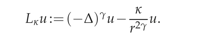
4 Hardy type operators with fractional Laplacian

Fix a constant κ∈R. Here we give a formula for the Green’s function for the Hardy type operator in Rn

In the light of Section 2, it is useful to use conformal geometry to rewrite the fractional Laplacian on Rnin terms of the conformal fractional Laplacian Pγon the cylinder M=R×Sn−1. Indeed,from the conformal property(2.3),setting

we have

Our aim is to study invertibility properties for the equation

Now consider the projection of Eq. (4.1)over spherical harmonics: if we decompose

then for m=0,1···,wm=wm(t)is a solution to

Recall Proposition 2.1 (taking into account that Q0=0). Then, in Fourier variables, Eq.(4.2)simply becomes

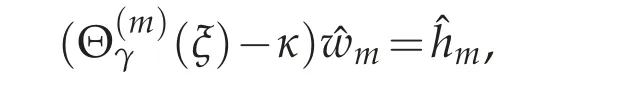
where

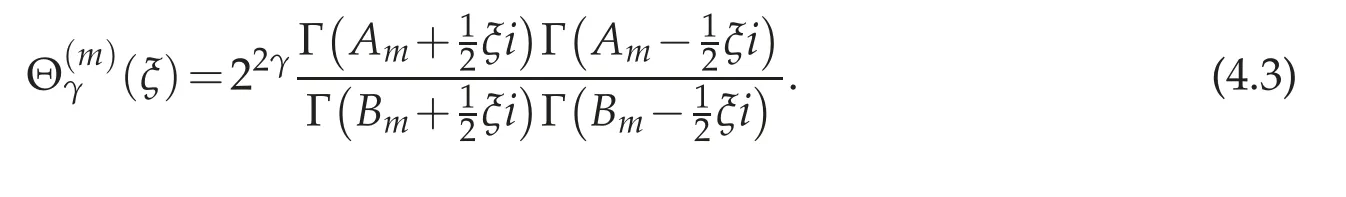
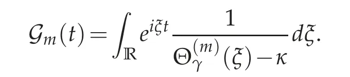
The behavior of the equation depends on the zeroes of the symbol(ξ)−κ. In any case,we can formally write

where the Green’s function for the problem is given by

This statement is made rigorous in [5] (see Theorem 4.2 below). First, observe that the symbol(4.3)can be extended meromorphically to the complex plane;this extension will be denoted simply by

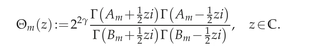
Remark 4.1. It is interesting to observe that Θm(z)=Θm(−z),and that,for ξ ∈R,

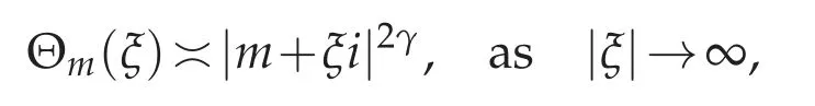
and this limit is uniform in m. This also shows that,for fixed m,the behavior at infinity is the same as the one for the standard fractional Laplacian(−∆)γ.

There are several settings depending on the value of κ. Let us start with the stable case.

Theorem 4.1([5]). Let 0≤κ<Λn,γand fix a non-negative integer m. Then the function

is meromorphic in z ∈C. More precisely, its poles are located at points of the form τj±iσjand−τj±iσj,where σj>σ0>0 for j=1,···,and τj≥0 for j=0,1,···. In addition,τ0=0,and τj=0 for all j large enough. For such j,{σj}is a strictly increasing sequence with no accumulation points.

Now we go back to problem(4.2). From Proposition 4.1 one immediately has:

Corollary 4.1. For any fixed m,all solutions of the homogeneous problem Lmw=0 are of the form

In the next section,we will give a variation of constants formula to construct a particular solution to(4.2). As in the usual ODE case,one uses the solutions of the homogeneous problem as building blocks.

4.1 The variation of constants formula

Before we state our main theorem,let us recall a small technical lemma:

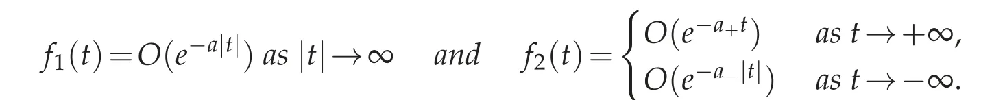
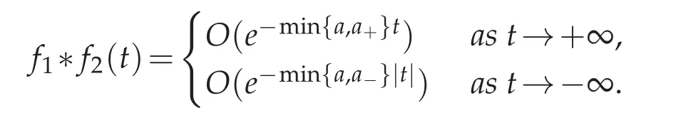
Lemma 4.1([5]). Suppose for a>0,a+a+>0,a+a−>0,a/=a+,a/=a−.‡‡When a=a+,the upper bound is worsened to O(te−at). A similar bound holds when a=a−.Then

From now on, once m=0,1,··· has been fixed, we will drop the subindex m in the notation if there is no risk of confusion. Thus,given h=h(t),we consider the problem

The variation of constants formula is one of the main results in[5]. Our version here is a minor restatement of the original result,to account for clarity. In addition,the proof has been simplified,so we give the complete arguments for statement(b)below.

Theorem 4.2 ([5]). Let 0 ≤κ<Λn,γand fix a non-negative integer m. Assume that the right hand side h in(4.4)satisfies for some real constants δ,δ0>−σ0. It holds:

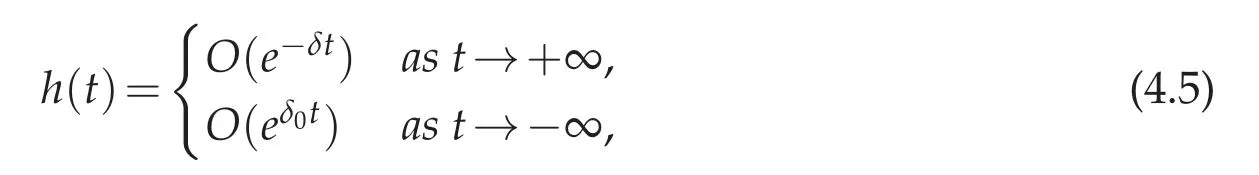
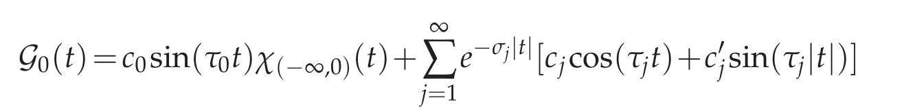
(a) A particular solution of (4.2)can be written as where

for some precise real constants cj,depending on κ,n,γ. Moreover, Gmis an even C∞function when t/=0.

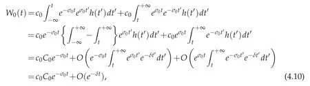
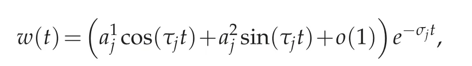
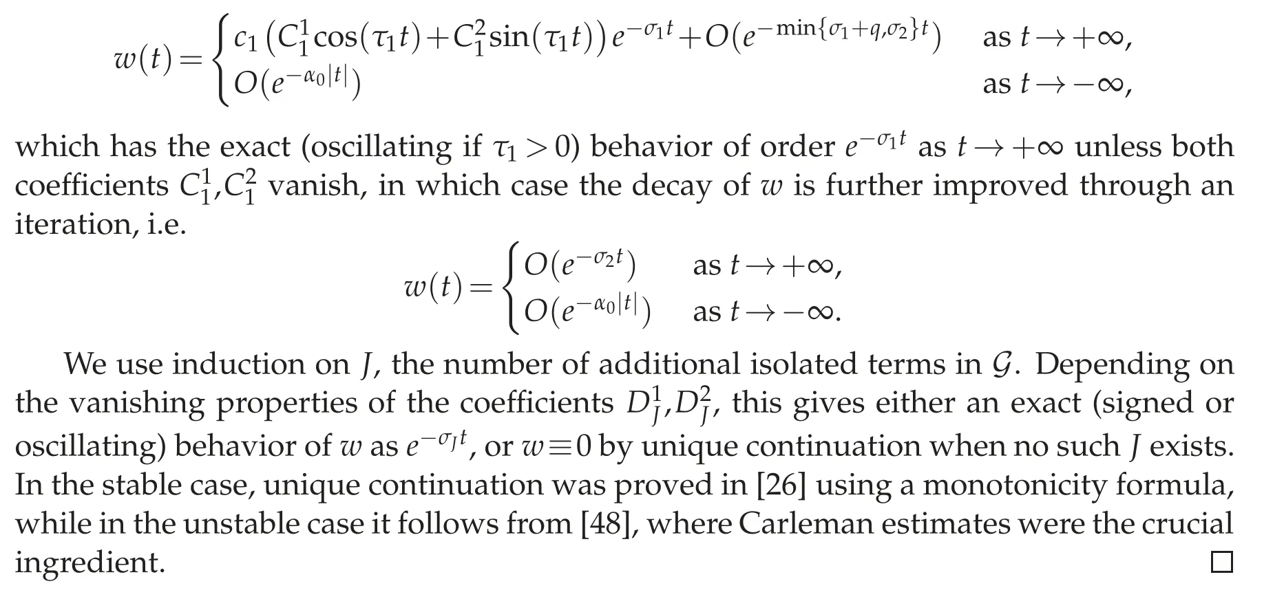
(b) Suppose δ>σJfor some J=0,1,···. Then the particular solution given by(4.6)satisfies

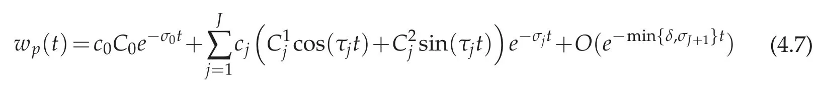
as t→+∞,and

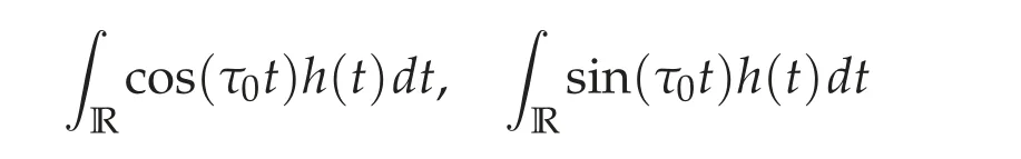
as t→−∞,where

and for each j=1,2,...,

Proof. The formula for the Green’s function Gmin (a) follows directly from [5]. We will prove(b),building on the first part. Without loss of generality we fix m=0 and suppress the subscript.

Note that G=O(e−σ0|t|)as t→±∞. Then,since δ,δ0>−σ0,Lemma 4.1 implies that,as t→−∞,

As for t→+∞,let us write

where

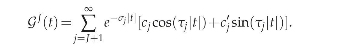
The particular solution in(4.6)is then given by

for

By Lemma 4.1, using the facts that GJ=O(e−σJ+1|t|) as t →±∞, δ>σJ>−σJ+1and δ0>−σ0>−σJ+1,we have

Next we turn to the terms W0and Wj,j=1,...,J. Their estimates are the same in spirit but that for W0is simpler since τ0=0.Using that δ>σJ>σ0and δ0>−σ0,we have eσ0·h∈L1(R)and we can write as t →+∞. Similarly, for all j=1,...,J, we have eσj·h ∈L1(R) in view of δ>σJ≥σjand δ0>−σ0. We can therefore compute

We also look at the case when κ leaves the stability regime. In order to simplify the presentation,we only consider the projection m=0 and the equation Moreover,we assume that only the first pole leaves the stability regime,which happens if Λn,γ<κΛn,γ. Then,in contrast to Theorem 4.1,we will have two additional real poles τ0and −τ0.

Proposition 4.1. Let Λn,γ<κ<. Assume the decay condition(4.5)for h as in Theorem 4.2. It holds:

(i) If δ,δ0>0,then a particular solution of(4.12)can be written as

where

for some constants cj,j=0,1,···. Moreover,G0is a C∞function when t/=0.

(ii) The analogous statements to Theorem 4.2(b),and Corollary 4.1 hold.

As we have mentioned, Theorem 4.2 can be interpreted in terms of the variation of constants method.This in turn allows the reformulation of the non-local problem(4.4)into an infinite system of second order ODE’s. Since the theory is particularly nice when all the τjare zero,we present it separately from the general case,in which complex notations are used.

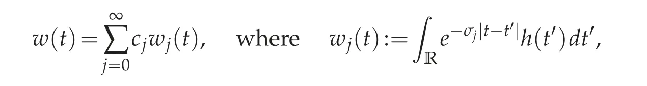
Corollary 4.2. Take w as in(4.6)from Theorem 4.2. In the special case that τj=0 for all j,then

where

Moreover,wjis a particular solution to the second order ODE

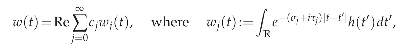
In general, such w can be written as a real part of a series whose terms solve a complex-valued second order ODE.

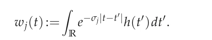
Corollary 4.3. Given w as in(4.6),we define the complex-valued functions wj:R→C by

They satisfy the second order ODE

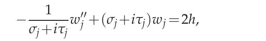
and the original(real-valued)function w can be still recovered by

Another interesting fact is that,for κ=0,equation(4.6)is simply the expansion of the Riesz potential for the fractional Laplacian. Indeed, let us recall the following (this is a classical formula;see,for instance,[13]and the references therein):

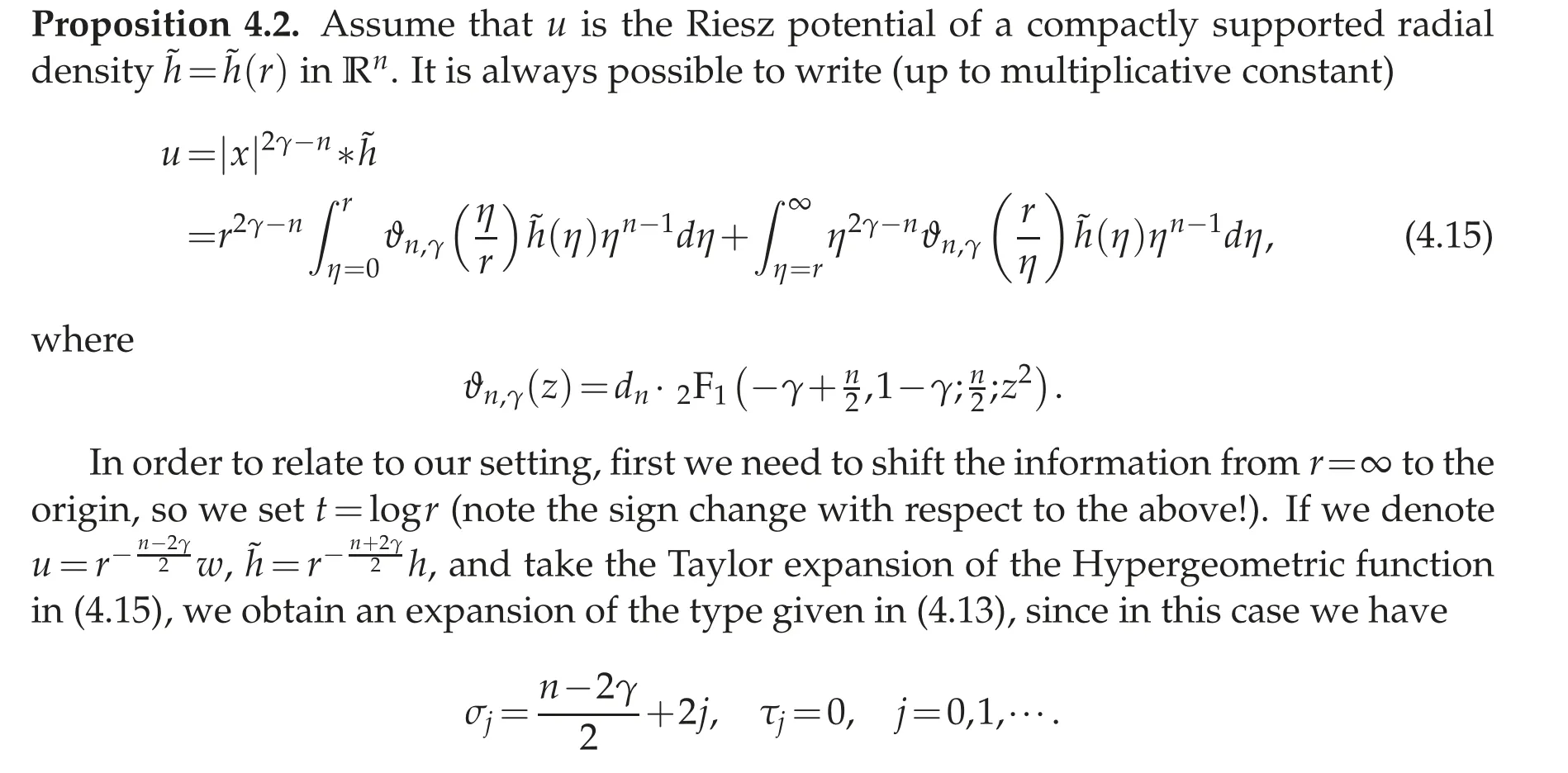
Thus we can interpret(4.13) as the generalization of(4.15)in the presence of a potential term with κ/=0.

4.2 Frobenius theorem

In the following, we will concentrate just on radial solutions (which correspond to the m=0 projection above),but the same arguments would work for any m. In particular,we study the kernel of the fractional Laplacian operator with a radially symmetric Hardytype potential,which is given by the non-local ODE

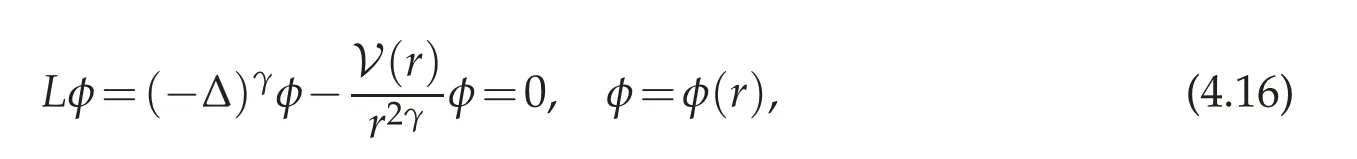
We have shown that this equation is equivalent to

where we have denoted φ=r−n−2γ2w,r=e−t.

The arguments here are based on an iteration scheme from [5] (Sections 6 and 7).However,the restatement of Theorem 4.2 that we have presented here makes the proofs more transparent,so we give here full details for convenience of the reader.

Assume,for simplicity,that we are in the stable case,this is,in the setting of Theorem 4.2. In the unstable case,we have similar results by applying Proposition 4.1.

We fix any radially symmetric,smooth potential V(t)with the asymptotic behavior

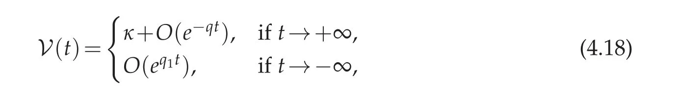
for some q,q1>0,and such that 0≤κ<Λn,γ.

The indicial roots for problem(4.17)as t→+∞are calculated by looking at the limit problem

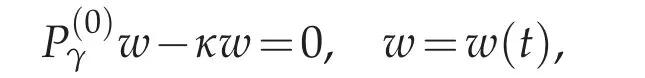
which are given in Theorem 4.1. Indeed,these are of the form

The results from the previous section imply that the behavior of solutions to (4.17)are governed by the indicial roots of the problem. This is a Frobenius type theorem for a non-local equation.

Proposition 4.3 ([5]). Fix any potential V(t) as above. Let w=w(t) be any solution to(4.17) satisfying that w=O(e−α0|t|) as |t|→∞for some α0>−σ0. Then there exists a non-negative integer j such that either

for some real number aj/=0,or

We remark that a similar conclusion holds at −∞.

Proof. Write the equation satisfied by w(4.17)as

Note that,by(4.18),

We follow closely the proof of Theorem 4.2 but, this time, since the right hand side h depends on the solution w,we need to take that into account in the iteration scheme. By part(a),a particular solution wp=G∗h satisfies

This is in fact the behavior of w, since the addition of any kernel element would create an exponential growth of order at least σ0which is not permitted by assumption. As a consequence,we obtain a better decay of w as t→+∞,so we can iterate this argument to arrive at

Using Theorem 4.2(b)with J=0,we have(in its notation)

When C0/=0,we have that

for a non-zero constant a0=c0C0.

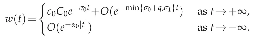
Otherwise,in the case C0=0,we iterate this process to yield

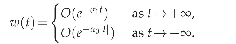
An application of Theorem 4.2(b)with J=1 yields

5 Non-degeneracy

The linearized operator is now

for the potential

for some q,q1>0.

Now we look for radially symmetric solutions to

which,in terms of the t variable,is equivalent to

Recall that the potential V∗is given in(5.1)and it is of the type considered in Proposition 4.3,so we know that the asymptotic expansion of solutions are governed by the indicial roots of the problem. These are given by:

Lemma 5.1([5]). Consider the equation(4.17)for the potential V∗as in(5.1). Then:

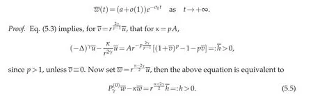
which is a solution of

Instead of the fractional Laplacian(−∆)γwe prefer to use the shifted operator(2.3)and thus we set

Then:

Proposition 5.1. There exists a>0 such that

Now,since w(t)decays both as t→±∞,we can use Proposition 4.3,taking into account that a0(or equivalently,C0from(4.8))cannot vanish due to(5.5).

Now we go back to problem(5.2). First, since (3.4) is invariant under rescaling, it is well known that

belongs to the kernel of L∗. We will show that this is the only possibility(non-degeneracy of u∗).

Set w∗defined as w∗=rn−2γ2φ∗. It is a radially symmetric,smooth solution to L∗w=0 that decays both as t→±∞. In particular,from Proposition 5.1 one has

for some a/=0.

5.1 Wro´nskians in the non-local setting

We will show that u∗is non-degenerate, this is, the kernel of L∗consists on multiples of φ∗. For simplicity, we will concentrate just on radial solutions (which correspond to the m=0 projection above), but the same argument would work for any m. Also,let us restrict to the stable case in order not to have a cumbersome notation. The main idea is to write down a quantity that would play the role of Wro´nskian for a standard ODE.We provide two approaches: first, using the extension (Lemma 5.2) and then working directly in Rn(Lemma 5.3).

Lemma 5.2. Let wi=wi(t),i=1,2,be two radially symmetric solutions to L∗w=0 and set Wi,i=1,2,the corresponding extensions from Proposition 2.3. Then,the Hamiltonian quantity

is constant along trajectories.

Proof. The proof is the same as the one from Theorem 3.1. however, we present it for completeness. By straightforward calculation, using (2.5) for the second equality and integrating by parts in the third equality,

since both w1and w2satisfy the same equation L∗w=0.

Now define the Wro´nskian of two solutions for the ODE(4.14)

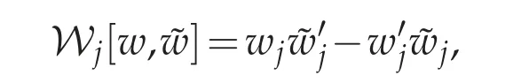
and its weighted sum in j=0,1,···

for the constants given in Theorem 4.2.

Lemma 5.3. Let w, ˜w be two radially symmetric solutions of L∗w=0. Then the Wro´nskian quantity from(5.6)satisfies

Proof. Just recall the ODE system formulation(4.13)and(4.14),consider the corresponding Wro´nskian sequence and sum in j. Since w and ˜w both satisfy

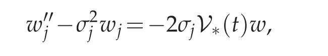
we see that

and the conclusion follows.

Proposition 5.2. Any other radially symmetric solution to L∗w=0 that decays both at±∞must be a multiple of w∗.

Proof. The proof is standard as is based on the previous Hamiltonian identities,applied to w and w∗. Let us write the proof using Lemma 5.3,for completeness.It holds

We claim that w and w∗must have the same asymptotic expansion as t→+∞. By Proposition 4.3, the leading order terms of w and w∗as t →+∞must be an exponential with some indicial root,i.e.

Since

we obtain that σj0=σj∗0. From the bilinearity of W[w,w∗],we can assume by rescaling that

aj0=aj∗0=1.

We now look at the next order. We suppose

for some complex numbers α,α∗with Reα,Reα∗≥j0and non-zero real numbers aα,aα∗. A direct computation of the Wro´nskian yields

In order that W[w,w∗]≡0, the next order exponents α and α∗must be matched and the same expression also tells us that aα=aα∗.

Inductively we obtain that, once w and w∗are rescaled to match the leading order,they have the same asymptotic expansion up to any order,as t→+∞. Unique continuation,as applied in the above results,yields the result.

5.2 The unstable case

Let us explain the modifications that are needed in the above for the unstable case. We consider only radially symmetric solutions(the m=0 mode).

First we recall some facts on the indicial roots as t→+∞. It holds that σ0=0, τ0/=0.We also know that σj>0 for all j ≥1, and τj=0 for all j ≥J, for some J large enough. A more precise estimate for J would be desirable,but it would be too technical.

Proposition 5.3. Let κ be as in Proposition 4.1 and w be as defined by(5.4). As t→+∞,either

Proof. We follow the ideas in Proposition 4.3. Note that if the integrals

do not vanish simultaneously,we have(i), while if both are zero, then we need to go to(ii). But this process must stop at J since aJis not zero again by(5.5),and we have(iii).

Note that a similar result has been obtained by [38] for γ=1/2, in the setting of supercritical and subcritical solutions with respect to the Joseph-Lundgren exponent pJL(corresponding to the stable and unstable cases here respectively).

6 Pohoˇzaev identities

Pohoˇzaev identities for the fractional Laplacian have been considered in [24,28,47], for instance. Based on our study of ODEs with fractional Laplacian, here we derive some(new)Pohoˇzaev identities for w a radially symmetric solution of

Here κ is a real constant. For later purposes,it will be convenient to replace

This equation appears,for instance,in the study of minimizers for the fractional Caffarelli-Kohn-Nirenberg inequality[6].

By Proposition 2.3,problem(6.1)is equivalent to

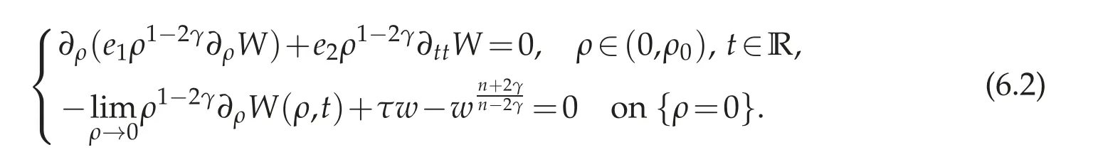
Proposition 6.1. If W=W(t,ρ)is a solution of(6.2),then we have the following Pohoˇzaev identities:

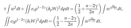
Proof. Multiply the first equation in(6.2)by W and integrate by parts;we have

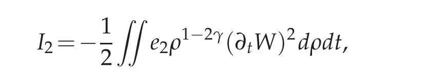
Next we multiply the same equation by t∂tW;one has

First we consider I1,

Here we have used e(ρ)→1 as ρ→0,and the second equation in(6.2). Similarly,it holds that

so we have

Combining(6.3)and(6.4),one proves the claim of the Proposition.

Now we provide another Pohoˇzaev type identity based on the variation of constants formula. We discuss first the simpler case where all τj=0,then the general case. Let w be a solution to(6.1). As in Corollary 4.2,we write w as

Proposition 6.2. Let w be a(decaying)radially symmetric solution to(6.1). Then

Proof. We multiply the above equation(6.5)by cjwj/σj,sum in j and integrate by parts:

Similarly,multiply the same equation by/σj,sum in j and integrate:

We add and subtract the two equations,to obtain

and

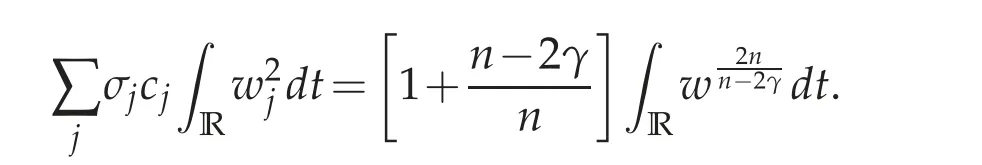
This completes the proof.

In the general case,as in Corollary 4.3,we write

Proposition 6.3. Let w be a(decaying)radially symmetric solution to(6.1). Then

Proof. The proof stays almost the same as in Proposition 6.2,except that we take real parts upon testing against the corresponding multiple of wjand tw′j,which yields

and

It suffices to add and subtract in the same way.

Acknowledgments

M.Fontelos is supported by the Spanish government Grant No. MTM2017-89423-P. The research of A. DelaTorre (partially) and M.d.M. Gonz´alez is supported by the Spanish government Grant No. MTM2017-85757-P. The research of J.Wei is supported by NSERC of Canada, and H. Chan has received funding from the European Research Council under the Grant Agreement No. 721675 “Regularity and Stability in Partial Differential Equations(RSPDE)”.