A FAST AND HIGH ACCURACY NUMERICAL SIMULATION FOR A FRACTIONAL BLACK-SCHOLES MODEL ON TWO ASSETS∗†

Hongmei Zhang Fawang Liu Shanzhen Chen Ming Shen

(1. College of Mathematics and Computer Science, Fuzhou University,Fuzhou 350108, Fujian, PR China;2. School of Mathematical Sciences, Queensland University of Technology,Qld. 4001, Australia;3. School of Economic Mathematics, Southwestern University of Finance and Economics, Chengdu 611130, Sichuan, PR China)

Abstract In this paper,a two dimensional(2D)fractional Black-Scholes(FBS)model on two assets following independent geometric L´evy processes is solved numerically. A high order convergent implicit difference scheme is constructed and detailed numerical analysis is established. The fractional derivative is a quasidifferential operator, whose nonlocal nature yields a dense lower Hessenberg block coefficient matrix. In order to speed up calculation and save storage space, a fast bi-conjugate gradient stabilized (FBi-CGSTAB) method is proposed to solve the resultant linear system. Finally, one example with a known exact solution is provided to assess the effectiveness and efficiency of the presented fast numerical technique. The pricing of a European Call-on-Min option is showed in the other example, in which the influence of fractional derivative order and volatility on the 2D FBS model is revealed by comparing with the classical 2D B-S model.

Keywords 2D fractional Black-Scholes model; L´evy process; fractional derivative;numerical simulation;fast bi-conjugrate gradient stabilized method

1 Introduction

During the last few decades the scientists have had a considerable interest in modelling financial markets and pricing financial derivatives. The pioneering work was presented in the 1970s by Black, Scholes [4] and Merton [23], who set up the key principles of no arbitrage option pricing and derived a well known differential equation model, that is the B-S model. However, the model was proposed under many strict assumptions on the real financial market. More general models by relaxing some restrictions were constructed in ongoing researches [12,13,24].

It is frequently found that the option price presents the features of heavy tails and volatility skew or smile in real markets. Gaussian models fail to describe these phenomena while L´evy (orα-stable) distributions can do. L´evy processes allow extreme but realistic events, such as sudden jumps of market prices [7,19,20]. Therefore,more and more different L´evy processes have been introduced into the financial field to model price of financial derivatives. A modified L´evy-α-stable process was proposed by Koponen [17] and Boyarchenko and Levendorskiˇi [5] to model the dynamics of securities. This modification yields a damping effect in the tails of the L´evy stable distribution, which was known as the KoBoL process. Carr, Geman,Madan and Yor[6]raised a L´evy process(that is the CGMY process),which allowed for jump components displaying both finite and infinite activity and variation. A finite moment log stable (FMLS) process with the tail indexα ∈(0,2], which can capture the highly skewed feature of the implied density for log returns,was applied to model S&P 500 option prices by Carr and Wu [7]. Schoutens [27,28] summed up the application of L´evy process in finance. Of all the L´evy processes, the most interesting include the CGMY, KoBoL and FMLS processes.

Fractional derivatives are quasi-differential operators, which provide useful tools for a description of memory and hereditary properties and are closely related to L´evy processes. When the price log-returns are driven by a L´evy fractional stable distribution,after some suitable transformations,the price of an option on underlying assets can be modeled by a fractional partial differential equation (FPDE) [1,8–10,14,34].In this paper we focus on a 2D FBS model governing European Call-on-Min option.Assuming the two underlying assetsS1andS2follow two independent geometric L´evy processes with maximal negative asymmetry (or skewness) [7] (that is the FMLS process), the option priceVon these two assets is determined by a 2D FBS equation [11] as below

wherex= lnS1, y= lnand the parametersrandσ(≥0) are the risk-free rate and the volatility of the returns from the holding stock price, respectively. The fractional operators(1<α,β≤2) are the left Riemann-Liouville fractional derivatives defined on infinite intervals [25]. Obviously, the FBS model (1) becomes the classical B-S model whenα=β=2.

It is well known that it is difficult to derive an analysis solution for FPDE.So numerical simulation of the fractional pricing model has attracted considerable attentions [3,8,10,15,21,32,33]. These financial literatures are all concerned with one-dimensional situations on one asset. As far as the author knows,the exploration of high dimensional fractional pricing model on multi assets is still sparse. Chen[11]used a finite different scheme to solve model (1) and price the Call-on-Min and Basket options approximately. Karipova and Magdziarz [16] derived a subdiffusive B-S model for the fair price of basket options by the optimal martingale measure and used the approximate methods to compare the classical with subdiffusive prices.

The non-locality of the fractional derivative operator leads to the denseness of coefficient matrices, which makes the solution of the discrete system more difficult.Moreover,the financial markets are becoming more and more complex,with trading of numerous types of financial derivatives. The market requires updated information about the values of these derivatives every second of the day. These yield a huge demand for feasible, fast and high accuracy numerical simulations. In this paper, a new implicit numerical scheme with second-order accuracy is constructed to approximate the above 2D FBS model in finite intervals. Due to the non-local nature of the fractional derivative, the numerical discretization of the 2D FBS model results in a linear system with a dense lower Hessenberg block coefficient matrix, which needs high storage space and computational requirement. This is disadvantageous in the face of huge financial data and ever-changing financial market. In order to speed up calculation and save storage space, the FBi-CGSTAB method is presented to evaluate the linear system. It would be a contribution to a real world problem whose solution would otherwise have been hampered by the fact that the solution of the partial differential equation is required in a short period of time.

The rest of the paper is structured as follows: Section 2 derives a fully implicit difference scheme (FIDS) with second order accuracy in both temporal and spatial directions when the price of two underlying assets is limited to finite intervals. The detailed numerical analysis is established in Section 3. In Section 4,a fast algorithm combining the bi-conjugate gradient stabilized method with the fast fourier transform is utilised to solve the discrete system in order to reduce the storage memory and computational cost. A numerical experiment with an exact solution is proposed in Section 5 to value the effectiveness and efficiency of the proposed fast numerical technique. Compared with the classical B-S model, the influence of fractional derivative order and volatility on the 2D FBS model is revealed in another example.The last section is dedicated to conclusions.

2 The Fully Implicit Difference Discretization

In the section, a FIDS for the 2D FBS model is constructed. In computation,we truncate the infinite solution domain into finite domain Ω = (xmin,xmax)×(ymin,ymax). Moreover, in order to facilitate the verification of the accuracy of the numerical scheme, we consider a more general form

with the following initial and boundary conditions:

Lemma 1[29]and its Fourier transform belongs toL1(R), then we have

uniformly for x ∈R, where p,q(p ̸=q)are integers andis the shiftedGr¨unwald-Letnikov difference operator[22]given by

with

Remark 1Considering a well defined functionu(x) on the bounded interval[a,b]. Ifu(a) = 0, the functionu(x) can be zero extended forx < a. Taking(p,q) = (1,0) in (4), theγ(1< γ ≤2) order left Riemann-Liouville fractional derivative ofu(x) at each pointxican be approximated by the following operator with second order truncation error

with

which satisfies [29]:

In the following we will construct a fully discrete scheme to approximate the equation (2). Lettn= (N −n)τ(n= 0,1,2,··· ,N) andxi=xmin+ihx, yj=ymin+jhy(i= 0,1,2,··· ,Mx;j= 0,1,2,··· ,My), whereτ=T/Nis a temporal step size,hx=(xmax−xmin)/Mxandhy=(ymax−ymin)/Myare spatial step sizes.We discretize the first-order spatial derivative by the central difference quotient and the R-L derivativesrespectively. As for the time derivative, the Crank-Nicolson scheme is employed. For simplicity, we define the following finite difference operators:

then equation (2) can be discretized as follows:

whose initial and boundary conditions is

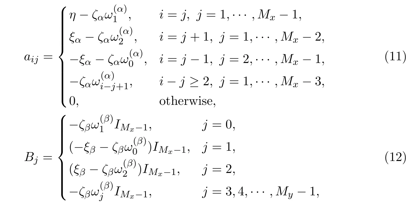
whereIis a unit matrix of order(Mx −1)×(My −1),Mis a block matrix which has(My −1)×(My −1)blocks and the size of each block matrix is(Mx −1)×(Mx −1),which is

where the matrixA=(ai,j)(Mx−1)×(Mx−1)has entries

and

with each block

Of course each (Mx −1)×(Mx −1) blochMi,jof the (My −1)×(My −1) block matrixMcan also be expressed by

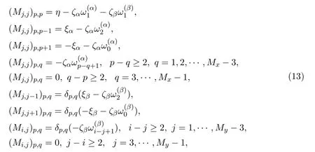
whereδp,qis the Kronecker delta.

3 Stability and Convergence of the FIDS

Using the Taylor expansion, we have

then the discrete scheme (6) can be transformed into

Similarly, the FIDS (7) can be transformed into

Let

where⊗is the Kronecker product,INis the identity matrix of orderN,(γ=αorβ) andDNare Toeplitz matrices of orderNwith the forms

Then the matrix form of the discrete scheme (15) is

Lemma 2[18]Let A ∈Rm×n, B ∈Rr×s, C ∈Rn×p, D ∈Rs×t, then

Moreover, if A,B ∈Rn×n, I is a unit matrix of order n, then matrixes I ⊗A and B ⊗I commute.

Lemma 3[18]For all matrices A and B,(A ⊗B)T=AT⊗BT.

Lemma 4[29]When1<γ ≤2, the eigenvalue λ of the matrixdefined in(13) satisfiesRe(λ)<0. Moreover, matrixis negative definite, and the realparts of the eigenvalues of the matrixare less than0, where

Lemma 5[18]Let A ∈Rn×n have eigenvaluesand B ∈Rm×m haveeigenvaluesThen the mn eigenvalues ofwhich represents the kro-necker product of matrix A and B, are

Lemma 6[26]Forbe the hermitian part of A and A∗be the conjugate transpose of A, then for any eigenvalue λ of A, it haswhereRe(λ)represents the real part of λ, λmin(H)and λmax(H)are respectively the minimum and maximum of the eigenvalues of H.

Theorem 1The FIDS(15)is unconditionally stable.

ProofAccording to Lemma 2, it has

then

which yields that any two of the matrices

can be commuted.

Therefore,

Calculate the symmetric form ofby Lemma 3 as:

Similarly,

According to Lemma 4, the real parts of the eigenvalues ofandare all negative for 1<α,β ≤2. Furthermore,from the consequences of Lemma 5 it has the real part of the eigenvalues ofandare all positive forLetλαandλβbe the eigenvalues of matricesrespectively,then the real parts ofλαandλβare both great than zero by Lemma 6. Since

are the eigenvalues of matrices

respectively,the spectral radius of these two matrices are both less than 1 forη >0,which yields that

converge to zero matrix whennapproximates to infinity. Therefore the FIDS (15)is unconditionally stable.

Proposition 1defined in(16)satisfy

where ∥·∥2is the2-norm.

ProofFrom the proof of Theorem 1, we know the real parts of the eigenvalues ofare all greater than 0. Furthermore,andare both real symmetric matrices, which yieldsandare positive definite.

For any real vectorv= (v1,v2,··· ,vMy−1)Twithvj= (v1,j,v2,j,··· ,vMx−1,j)(j=1,2,··· ,My −1) andη >0, we have

Substitutingvandin the above formula, respectively, it obtains

which leads to

Similarly, it can be obtained thatTherefore,

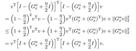
Moreover, according to the positive definiteness of matricesandfor any real vectorv, it gets

Then

which means

Consequently,

holds because of the commutativity of the matrices.

Similarly,

is valid. The proof is completed.

Theorem 2Letbe the exact solution of model(2)andbe the solutionof the discrete equation(15). Then for1<α,β ≤2, it obtains

where C is a positive constant.

ProofLetSubtracting (14) from (15) leads to

where

Then

where

Sinceaccording to Proposition 1 it gets

The proof is completed.

4 Fast Bi-conjugate Gradient Stabilized(FBi-CGSTAB)Method for Solving the FIDS

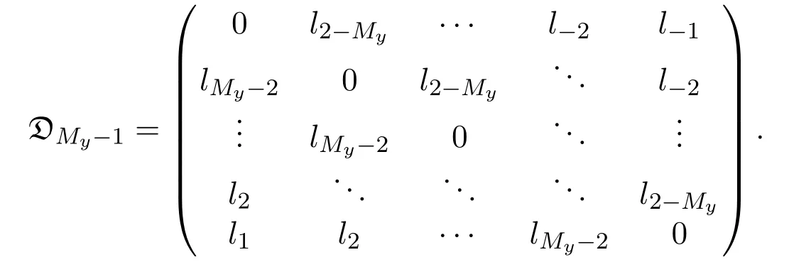
The implicit difference discretization of equation (2) results in a linear system with a dense lower Hessenberg block coefficient matrix. Solving the linear system(9) directly, such as by Gaussian elimination method, requires a computational cost ofper time step and storage memory ofwhich represents a high computational expense. Moreover, the ever-changing market information and enormous financial data lead to the complexity of the market. These urgently require fast computing. In the section, we present an efficient iterative method to solve(9)by combing the bi-conjugate gradient stabilized(Bi-CGSTAB)method[30]and fast Fourier transform(FFT),which significantly reduces the computational cost toO(MxMylog(MxMy)) per time iteration and the storage space toO(MxMy).

By a simple calculation,Min formula (9) can be decomposed as

According to the formulae (16) and (17), it only needs to storeinstead of the full matrixM. Moreover, the elements of the vectoralso need to be stored. Then the total memory requirement has been significantly reducedMx+My+2+(Mx −1)(My −1)=O(MxMy).

In the following, we consider the computational cost.

Since using the conjugate gradient squared method to solve the nonsymmetric linear system (9) may arise the irregular convergence patterns, in order to avoid the problem, the Bi-CGSTAB method is applied to (9) ([2,30]).

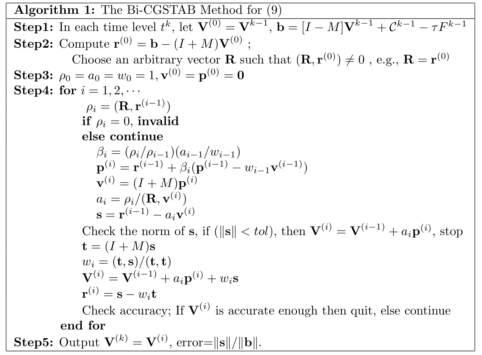
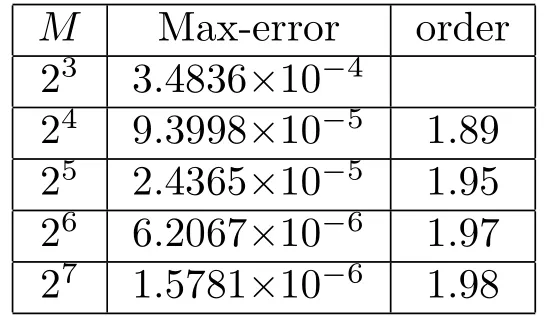
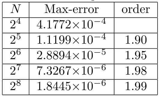
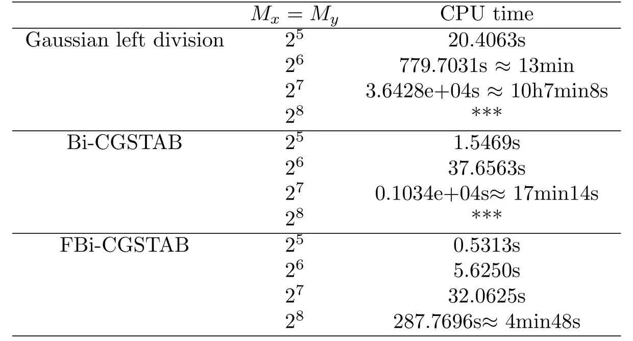
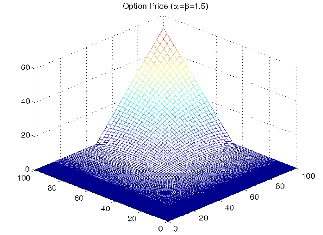
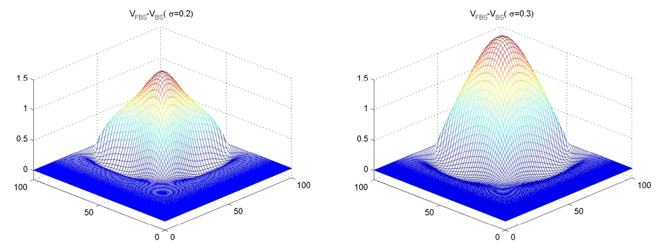
Algorithm 1: The Bi-CGSTAB Method for (9)Step1: In each time level tk, let V(0) =Vk−1, b=[I −M]Vk−1+Ck−1 −τFk−1 Step2: Compute r(0) =b −(I+M)V(0) ;Choose an arbitrary vector R such that (R,r(0))̸=0 , e.g., R=r(0)Step3: ρ0 =a0 =w0 =1,v(0) =p(0) =0 Step4: for i=1,2,···ρi =(R,r(i−1))if ρi =0, invalid else continue βi =(ρi/ρi−1)(ai−1/wi−1)p(i) =r(i−1)+βi(p(i−1)−wi−1v(i−1))v(i) =(I +M)p(i)ai =ρi/(R,v(i))s=r(i−1)−aiv(i)Check the norm of s, if (∥s∥

In Algorithm 1, in addition to the operation of matrix-vector multiplication, the computational costs of other operations are onlyO(MxMy), so we have to compute the matrix-vector multiplication in an efficient way (that is FFT) to reduce the computational complexity. Since the matricesare all Toeplitz matrices, and noting the decomposition in (16) and (19), we only need to consider the computational cost offor the Toeplitz matrix

where

Then the matrix-vector multiplication can be calculated as follows:

It is well known that the circulant matrixcan be decomposed as

wherecis the corresponding two dimensional FFT of the first column vector ofis the 2(M −1)×2(M −1) discrete Fourier transform matrix given by

for 1≤j,k ≤2(M −1)−2. For any vectorv, the matrix-vector multiplicationcan be carried out inO((Mx −1)(My −1)log(Mx −1)(My −1)) operations via the FFT (see [31]). Therefore, by FBi-CGSTAB method, the computational cost of solve linear system (9) has been significantly reduced toO(MxMylog(MxMy)) per time iteration.

5 Numerical Experiments

Example 1Consider the following fractional diffusion-convection-reaction equation with a source term

where the source term

The exact solution of this equation isV(x,t)=x3y4eT−t.

In Example 1, we always take the values of parameters asα=1.7, β=1.8, r=0.05, σ=0.25 andT=1.0.

Tables 1 and 2 list the errors in the maximum-norm and its corresponding convergence order of equation(20). From these tables,it can be seen that the numerical solution obtained by the FIDS (7) is very close to the exact solution. Furthermore,the convergence order of FIDS is in good agreement with the conclusion of Theorem 2. Here the convergence orders of the FIDS are computed by logfor the spatial step sizefor the temporal step sizerespectively. The notationerroricorresponds to the error whenh=hior ∆τ=∆τi.

M Max-error order 23 3.4836×10−4 24 9.3998×10−5 1.89 25 2.4365×10−5 1.95 6.2067×10−6 26 1.97 27 1.5781×10−6 1.98

N Max-error order 24 4.1772×10−4 25 1.1199×10−4 1.90 26 2.8894×10−5 1.95 27 7.3267×10−6 1.98 28 1.8445×10−6 1.99

The consumed CPU times to run the Gaussian left division method, the Bi-CGSTAB method and the FBi-CGSTAB method for fixed temporal stepτ=1/300 are respectively displayed in Table 3. Especially, for the Gaussian left division method and the Bi-CGSTAB method,the computer does not work properly because there is no sufficient storage space whenMx=My= 28. From which it can be seen that the FBi-CGSTAB method has significantly reduced the computational requirement and the storage space. We carried out all numerical computations by using MATLAB on Lenovo L430 laptop with configuration: Intel(R) Core(TM) i5-7500, 3.40GHz and 8.0G RAM.

Mx =My CPU time Gaussian left division 25 20.4063s 26 779.7031s ≈13min 27 3.6428e+04s ≈10h7min8s 28 ***Bi-CGSTAB 25 1.5469s 26 37.6563s 27 0.1034e+04s≈17min14s 28 ***FBi-CGSTAB 25 0.5313s 26 5.6250s 27 32.0625s 28 287.7696s≈4min48s

Example 2We now consider the following FBS model on two assets for a European Call-on-Min option

whereKis the strike price andTis the expiry time.

We use the FIDS(7)to solve this model approximately. Here taking the parameterK=50, T=1, r=0.05. The numerical results of the European Call-on-Min option are plotted in Figure 1 against the stock pricesS1= exandS2= eywithα=β=1.5 andσ=0.25, which shows a fat tail characteristics.

To illustrate the influence ofαandβon the option price, we calculate the price of European Call-on-Min option numerically for differentαandβ, and plot the difference curves between the numerical solutions of the FBS model (21) and the classical B-S model in Figure 2 att=0.

From Figure 2, one can see that the call option price obtained by FBS model increases asαandβdecrease when the stock pricesS1andS2are greater than a critical value ( but close to the strike price), which likely implies that the option price exhibits a jump (or convective) nature whenαandβare close to 1, the jump nature of the FMLS process delivers much higher prices. Whileαandβare close to 2, the corresponding option price mainly presents a diffusive nature. Furthermore,in order to observe the effect of volatility rateσon the option price, the difference curves for differentσare presented in Figure 3 whenα=β= 1.5. Figure 3 shows that the difference value increases as the volatility rateσincreases whenS1andS2are greater than a critical value,which suggests that the FBS model is more sensitive to volatility change compared with the classical B-S model. It would be indicated that the FBS model can better capture the dynamic process of option price changes.

6 Conclusion

The complexity of the financial markets and non-locality of the fractional derivative operator yield a huge demand for feasible, fast and high accuracy numerical simulations to FBS models. In the paper, a FIDS is constructed for a 2D FBS model, which is unconditional stable and second-order convergent. Then, in order to solve the resultant linear system quickly and effectively, a FBi-CGSTAB is presented which significantly reduces the computational cost toO(MxMylog(MxMy))per iteration and the storage space toO(MxMy). One numerical example with exact solution is chosen to confirm our theoretical analysis. The comparison of CPU time spent on running the Gaussian left division method, the Bi-CGSTAB mehtod and the FBi-CGSTAB method highlights the remarkable effectiveness of the FBi-CGSTAB in rapid computation. It is worth mentioning that this fast and high accuracy numerical technique can be applied to similar models.

A European Call-on-Min option is priced by the FBS model and the proposed numerical technique, which can also be used to price other more complex options,such as barrier options. For differentα,βandσ, the difference curves of option prices between the FBS model and the classical B-S model are plotted. From these graphical features, we may think that the FBS model based on the L´evy process not only presents the feature of fat tail, but also can capture some extreme but realistic events, such as sudden jumps of prices, and thus more correctly simulate the dynamics of option prices in markets with jumps than the classical B-S model.We believe that these findings provide useful information for further applications of the fractional calculus in financial market.