LONG-TERM DYNAMIC ANALYSIS OF ENDANGERED SPECIES WITH STAGE-STRUCTURE AND MIGRATIONS IN POLLUTED ENVIRONMENTS∗†

Fangfang Liu Kexin Wang Fengying Wei

(1. College of Mathematics and Computer Science, Fuzhou University, Fuzhou 350116,Fujian, PR China;2. Key Laboratory of Operations Research and Control of Universities in Fujian,Fuzhou University, Fuzhou 350116, Fujian, PR China)

Abstract We propose a stochastic stage-structured single-species model with migrations and hunting within a polluted environment,where the species is separated into two groups: the immature and the mature,which migrates from one patch to another with different migration rates. By constructing a Lyapunov function, together with stochastic analysis approach, the stochastic single-species model admits a unique global positive solution. We then utilize the comparison theorem of stochastic differential equations to investigate the extinction and persistence of solution to stochastic single-species model. The main results indicate that the species densities all depend on the intensities of random perturbations within both patches. As a consequence, we further provide several strategies for protecting endangered species within protected and unprotected patches.

Keywords protection zones; stage-structure; random perturbations; migration; extinction and persistence

1 Introduction

The establishment of the protection zones within some countries or areas around the world has been widely accepted and recognized as an efficient strategy to avoid the endangered species from extinction when faced the excessive activities of human beings. The researchers proposed and formulated the population models between unprotected and protected patches to investigate how the dynamic mechanics of the species undertook in the long run. For instance, Zou and Wang [2] studied the dynamic behaviors of a deterministic single-species model with diffusion between two patches

wherex(t) andy(t) respectively represent population densities of the species in unprotected and protected patches at timet,rmeans the intrinsic growth rate,Krefers to the carrying capacity of environments,dis the diffusion coefficient,Edenotes the hunting rate in unprotected patch. By assuming that the size of the unprotected patches isHand the size of the protected patches ish;the diffusion term is proportional to the differences of densities between two patches, by considering a size-dependent single-species model with migration and hunting, they derived that reducing the diffusion coefficient and increasing the size of the protection zone are both propitious for the enhancement of population levels within protected patch.Other latest results regarding the protection zones could be found in the literatures[4,13,21,31-34].

Pollution of environments often seriously threatens spaces for survival for most species on the globe. The fact is that, some species become extinction, and more species are endangered when they simultaneously face environmental and human pollution. Nowadays, it therefore is of especial importance to study the persistence and extinction for endangered species within polluted environments. Recently,many scholars have conducted extensive researches on endangered species regarding polluted environment and toxins distribution, and have obtained some good related results. For example, Srinivsu [26] studied a single-population model in which the input toxin is a constant, and obtained sufficient conditions for the consistence,persistence and extinction. Later, Yanet al.[27] found the criteria for survival and extinction by comparison theorem of ordinary differential equations to study the dynamic behaviors of a single-population model, when the population growth rate in the polluted environment is nonlinearly related to the toxin concentration in species. Almost at the same year, Yanget al.[28] investigated the persistence of a single-population model in polluted environment by Dulac function method, and obtained sufficient conditions for the global stability of positive equilibrium state to the model, and further explained its corresponding biological meaning.

We in this paper propose a single-species model in which the species moves between patches: unprotected patch and protected patch. We denote the density of individuals for endangered species in unprotected patch at timetbyx(t), and the density of individuals in protected patch byy(t). Thereinto, the matures within unprotected and protected patches are respectively denoted byxm(t)andym(t),and the immatures within unprotected and protected patches are respectively denoted byxi(t) andyi(t).

WWF China made fourth investigation upon outdoor survival of wild giant pandas in China from 2011 to 2014, which shows that, the number of wild giant pandas within mainland of China has reached 1864, and the number of giant pandas in protected patches has accounted for 66.8% within total number in mainland of China(see [36]). Another case in National Forestry and Grassland Administration and National Park Administration claimed that the number of South China tiger (also called Panthera tigris Amoyensiss in references)in protected patch has accounted for 55% of the total number within mainland of China (see [37]). For Tibetan antelope(referred also as Pantholops hodgsoniis), the number in protected patches has accounted for 70%of the national quantity(see[37]). Combined with the above cases,we here assume that the amount of individuals of endangered species in protected patch is larger than that in unprotected patch in this paper:

whereK1>1 andK2>1, and there is a certain proportional relationship between the immature and the mature in protected patch as follows:

with 0< K3<1, K4>1. We further assume that migration process for the mature is a double-direction activity due to the spread of toxicant, that is, the mature in unprotected patch would migrate from and to protected patch due to shortage of food-resource and concentration of toxicant. Then we reach the following delayed ordinary differential equations, which describe the single-species in a polluted unprotected patch with stage-structure and migration:

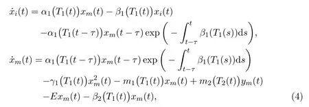
whereα1(T1) denotes the birth rate of the immature in unprotected patch;β1(T1)andβ2(T1) denote the death rates of the immature and the mature in unprotected patch respectively;γ1(T1) denotes the competition rate of the mature in unprotected patch;m1(T1) means the toxicant-dependent migration rate from unprotected to protected patch;m2(T2) stands for toxicant-dependent migration rate from protected to unprotected patch;Eis the hunting rate by human beings and hereT1(t)andT2(t) respectively mean toxicant concentrations in the environment at timetin unprotected and protected patches respectively.

For the mature in protected patch, the individuals would migrate from and to unprotected patch due to shortage of finding mate or survival resource or other possible reasons. Then we get the following delayed ordinary differential equations:

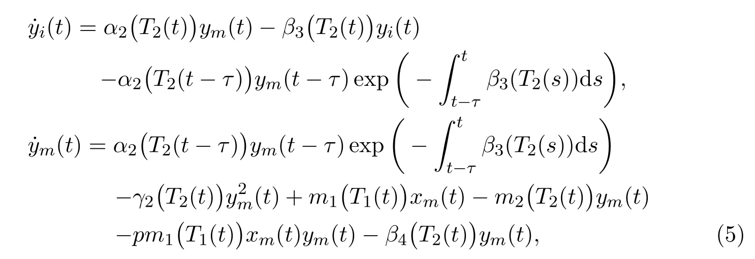
whereα2(T2) denotes the birth rate of the immature in protected patch;β3(T2)andβ4(T2) denote the death rates of the immature and the mature in protected patch respectively;γ2(T2) denotes the competition rate of the mature in protected patch;pm1(T1)xmymstands for the individuals poisoned with probabilitypthrough direct contacts by the mature individuals who carry toxicant migrating from unprotected patch.

Meanwhile, toxicant concentrations within unprotected and protected patches obey the following ordinary differential equations:

whereQi(t) (i= 1,2) are the emission rates of the toxicant into the environment, which are always assumed to be bounded non-negative functions oft, andQ1(t)≫Q2(t);δ1andδ2represent the natural washout rates of the toxicant in the environment;δ3,δ4,δ5andδ6are the depletion rates of the toxicant concentration in the environment due to the uptake by the immature and mature individuals in unprotected and protected patches, respectively. Equation (6) gives the boundedness of toxicant concentration by means of comparison theorem of ordinary differential equations hereMoreover, we always assume thatαi(Ti) (i= 1,2) are non-increasing functions of toxicant concentrations,β1(T1),β2(T1),β3(T2),β4(T2),γi(Ti) (i= 1,2) andmi(Ti) (i= 1,2) are nondecreasing functions of toxicant concentrations:

Throughout this paper, we denote notations as follows:

fori=1,2,j=1,2,3,4.

Thus we come to deterministic model within two patches as follows:

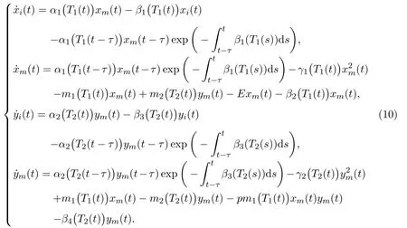
As all we know, the growth of any species in the real world is inevitably subject to random interference from external environments. Random interference could be roughly divided into two categories. One is the sum of many tiny and independent random disturbances, mathematically it is called white noise, such as small changes in temperature,humidity,wind and sunlight. The other is a small number of random disturbances with a large intensity. Then the growth rate of the objects will change greatly when this type of random disturbance occurs,which is usually called colored noise(not a pure white noise any more),such as cold wave,major earthquake,tsunami and volcanic eruption. In this paper, we mainly study the interference caused by white noise to a single-species (10). For simplicity, external interferences are put into model (10), and now, we start to focus on the stochastic single-species model with stage-structure and migrations within polluted environments, which takes the following form:

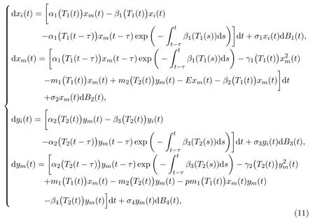
whereBi(t)(i=1,2,3,4)are mutually independent one-dimensional standard Brownian motions defined on the complete probability spacewith its filtrationsatisfying the usual conditions, andσi >0(i= 1,2,3,4) are the intensities of white noises in [15]. And, effects of toxicant on stochastic biological models were paid much attention by scholars around the world. For instance, in 2009, Liu and Wang [24] studied a stochastic single-population model in a polluted environment, using stochastic analysis methods to obtain sufficient conditions for random persistence, random mean weak persistence and local extinction, and random mean weak persistence as well. In 2010,Liu and Wang[25]studied a stochastic single-population model with Markov transformation in a polluted environment,and proved the average strong persistence, random persistence, random average weak persistence, extinction and other related results.

The initial conditions of model (11) are given as follows:

whereφi(ξ)(i= 1,2,3,4) are the continuous functions mapping from the interval[−τ,0] into [0,∞), and model (11) will work on the regionxi >0,xm >0,yi >0,ym >0}.

We attempt to organize this paper by several parts: We will prove that model(11)admits a unique global positive solution in the next section. The sufficient conditions guarantee the extinction and the persistence of the single-species within two patches which will be established respectively in Sections 3 and 4. As a consequence,we derive the conclusion of this paper and demonstrate several examples and their numerical simulations.

2 Existence and Uniqueness of Positive Solution

Theorem 2.1For any given initial data(12), there exists a unique solution(xi(t),xm(t),yi(t),ym(t))to model(11)on t ≥0and the solution will remain inwith probability one. That is,holds almost surely forall t ≥0.

ProofBy the approach mentioned in Maoet al.[15], we easily obtain that the coefficients of model (11) obey the local Lipschitz condition, hence model (11) has a unique local solution (xi(t),xm(t),yi(t),ym(t)) on [0,τe), whereτeis the explosion time. In order to show that the solution is global, it is sufficient to showτe=∞a.s.. Letk0≥1 be large enough such that forξ ∈[−τ,0],xm(ξ),ym(ξ),xi(0),yi(0)lie within the interval [1/k0,k0]. For each integerk > k0, we define the stopping time

Obviously,τkis an increasing function ask →∞. We denoteaccording to the definition of the stopping time and the fact thatτeis the explosion time,we derive thatτ∞≤τe. In order to prove the assertionτe=∞holds almost surely,we need to check thatτ∞=∞will be valid almost surely. Otherwise, there is a constantε ∈(0,1) such that P{τ∞<∞}>ε. Then, there exist an integerk1≥k0and a constantT0>0 satisfying P{τk ≤T0} ≥ε,for allk ≥k1. We define aC2-functionV:as follows:

whereaandbwill be determined below. The ItÔ’s formula then gives that

Here

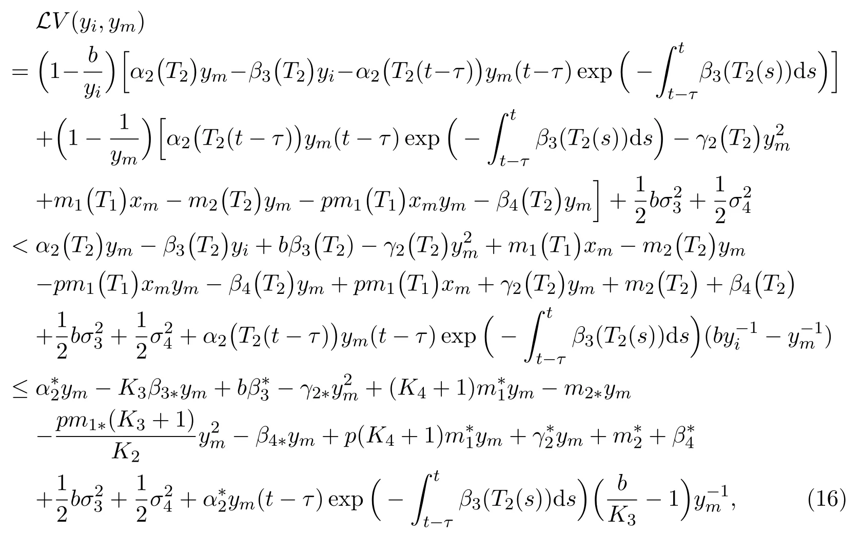
due to (2) and (3), and the fact that the last term of (16) vanishes when we chooseb=K3. So, we have

By similar discussion, we chooseaK1=1 and derive that

Combining (17) with (18) gives that

which is a polynomial with respect toxi,xm,yi,ym. Note that the coefficient of the first term is negative, then there exists a constantMsuch thatLV(xi,xm,yi,ym)≤M. We therefore obtain that

Integrating both sides of (20) from 0 toτk ∧T0, taking the expectation, one can get that

We set Ωk={τk ≤T0}fork ≥k1, then the probability given above turns into P{Ωk}≥ε. Note that forω ∈Ωk, each component of (xi(τk,ω),xm(τk,ω),yi(τk,ω),ym(τk,ω)) equals eitherkor 1/k, and hence

Therefore,

where a contradiction is derived when lettingk →∞. The proof is complete.

3 Extinction of Single-species within Patches

For a stochastic ecological system, we are always interested in its long-term behavior. In this section, we will analyze the extinction of the solution to model(11). The following definition of the extinction and two important lemmas will be widely used throughout our discussions.

Definition 3.1[16]A species is said to be extinct, if the population densityx(t)satisfies

Lemma 3.1[17]Suppose that a(t), b(t)and α(t)are bounded continuous functions defined on[0,∞), and a(t)>0, b(t)>0. For any initial value x(0)=x0>0,there exists a unique continuous solution x(t)to an equation

such that x(t)is global and represented by

Lemma 3.2[18]Consider a one-dimensional stochastic differential equation

Suppose that2a > σ2, and x(t)is a solution to(26)with any initial value x0>0,then the following results hold almost surely

Theorem 3.1If the parameters of model(11)satisfy

then the mature in protected patch tends to extinct, that is

ProofIntegrating both sides of the fourth equation in model (11), we thus derive

In order to eliminate terms with delay,we substitute(29)into right hand side of the following expression

which then gives that

due to (2) and (3). We simplify (31) into the following form

where

Let Ψ1(t) be a solution to the following SDE

with the initial value Ψ1(0) =C1, Lemma 3.1 implies that (34) admits a unique solution

where

Then the comparison theorem of stochastic differential equation yields

Theorem 3.2If the parameters of(11)satisfy

then the immature in protected patch tends to extinct, which means that0 a.s..

ProofBy assumption (3), the third equation of model (11) gives that

Let Ψ2(t) be a solution to the following linear SDE

with its initial value Ψ2(0)=yi(0), and the expression of whose solution is given by(see [17]):

The comparison theorem of stochastic differential equation yields that

By the similar discussion,we can obtain Theorems 3.3 and 3.4,in which sufficient conditions for the extinction of immature and mature individuals in unprotected patch are guaranteed.

Theorem 3.3If the parameters of model(11)satisfy

then the mature in unprotected patch is extinct, that is

Theorem 3.4If the parameters of model(11)satisfy

then the immature in unprotected patch is extinct, that is

Remark 3.1What we concern in this paper is what conditions will lead to the extinction of single-species within two patches. To avoid the extinction of singlespecies, we state our main results from the following aspects: the migration rates,the hunting rates and the birth/death rates as well.

First of all, the migration rates of single-species between two patches are the important indicators. Indeed, we could see how the migration rates work for the extinction of single-species when other parameters are fixed. Here, the sufficient condition of Theorem 3.1 demonstrates that the increasing ofor the decreasing ofwill lead to the extinction of the mature individuals in the protected patch, when the perturbation of the mature in protected patchσ4is fixed. On the contrary, Theorem 3.3 implies that the decreasing ofdsand the increasing ofcan make the mature individuals in unprotected patch extinct, when other parameters are fixed.

Further, the hunting rate in Theorem 3.3 also makes sense in order to avoid the extinction for the mature individuals in the unprotected patch. Here say, the larger the hunting rateEis, the more easily the mature individuals tend to extinction.That is, the decreasing of hunting rate effectively avoids the extinction of singlespecies.

As we mentioned above, the birth/death rates play vital roles when the extinction of the mature individuals and immature individuals is investigated. Theorems 3.1 and 3.2 demonstrate that the decreasing ofand the increasing oftogether withwill tend to the extinction of single-species in protected patch.

4 Persistence of Species within Patches

In this section,some results about the persistence of the species in protected and unprotected patches are achieved.

Definition 4.1[29]A species is said to be strongly persistent in the mean, if the population densityx(t) satisfies

Definition 4.2[31]A species is said to be strongly persistent, if the population densityx(t) satisfies

Next, we will discuss the sufficient conditions for the persistence of the mature and immature individuals in protected patch, respectively. In order to analyze the persistence of the mature in protected patch,we need to show a property in advance as presented in Lemma 4.1.

Lemma 4.1Let(xi(t),xm(t),yi(t),ym(t))be a solution of model(11)with any initial condition(12), we then derive that

ProofApplying ItÔ’s formula to the fourth equation of (11), we can obtain

Integrating both sides of (48) from 0 totyields that

whereθ >1,γ >1. For almost allω ∈Ω, there exists ak0(ω), by Borel-Cantelli Lemma, for allk ≥k0(ω), such that

Recall the fact that, in the real world, the amount of mature individuals in protected patch will not increase rapidly within a time interval, say here [t −τ,t],and will not and to zero soon. We therefore assume that mature individuals in protected patch admits certain proportional relationship as follows:

where 0< K5<1 andK6>1. Substituting (50) into (49), together with (2), (3),(9) and (51), we can get

Let

where

Obviously,the functionf(ym)is monotonically increasing in(0,1/D2),monotonically decreasing in(1/D2,∞),sof(ym)takes its maximum at 1/D2. For all 0≤s ≤γkandym >0, there exists aCindependent ofksuch that

Ifγ(k −1)≤t ≤γkandk ≥k0(ω), we have

Letk →+∞(that is,t →+∞), we therefore have

By the similar argument, one derives that

The proof is now complete.

Theorem 4.1If the parameters of(11)satisfy

then the mature in protected patch is strongly persistent in the mean, and satisfies the following property

ProofApplying ItÔ’s formula to the fourth equation of (11), we derive that

Integrating both sides of (61), and together with (2), (3), (51) as well as (9), we have

The strong law of large numbers for martingales yieldsTogether with Lemma 4.1, under condition (59), we finally achieve that

The proof is complete.

Theorem 4.2If the parameters of model(11)satisfy the following condition

then the immature in protected patch is strongly persistent.

ProofAccording to the similar approach given in Theorem 3.1, we derive the following inequality

Taking integration on both sides of (64), yields that

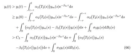
In order to eliminate terms with delay, we consider

where

We therefore have the following inequality

Further, the comparison theorem of stochastic differential equation gives that

and the strong law of large numbers for martingales also givesUnder condition (63), we can getThe proof is complete.

According to the same approaches,we can obtain that solutions of the immature and mature in unprotected patch respectively are strongly persistent and strongly persistent in the mean. Then we can obtain the following theorems.

Theorem 4.3If the parameters of(11)satisfy

then the mature in unprotected patch is strongly persistent in the mean and has the property

Theorem 4.4If the parameters of model(11)satisfy the following condition

then the immature in unprotected patch is strongly persistent, which means that

5 Examples and Simulations

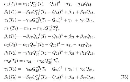
Several examples and the corresponding numerical simulations will be presented to support the main results by means of Milstein Method [23]. Now, consider the linear case of model (11):

and the nonlinear case of model (11):

which are shown in Figure 1.

Now, hereafter, in model (11) we letK1=K2= 4,K3= 0.8,K4= 1.2,K5=0.9,K6=1.1,τ=1,p=0.5 in this section. And, we come to two illustrative examples as follows.

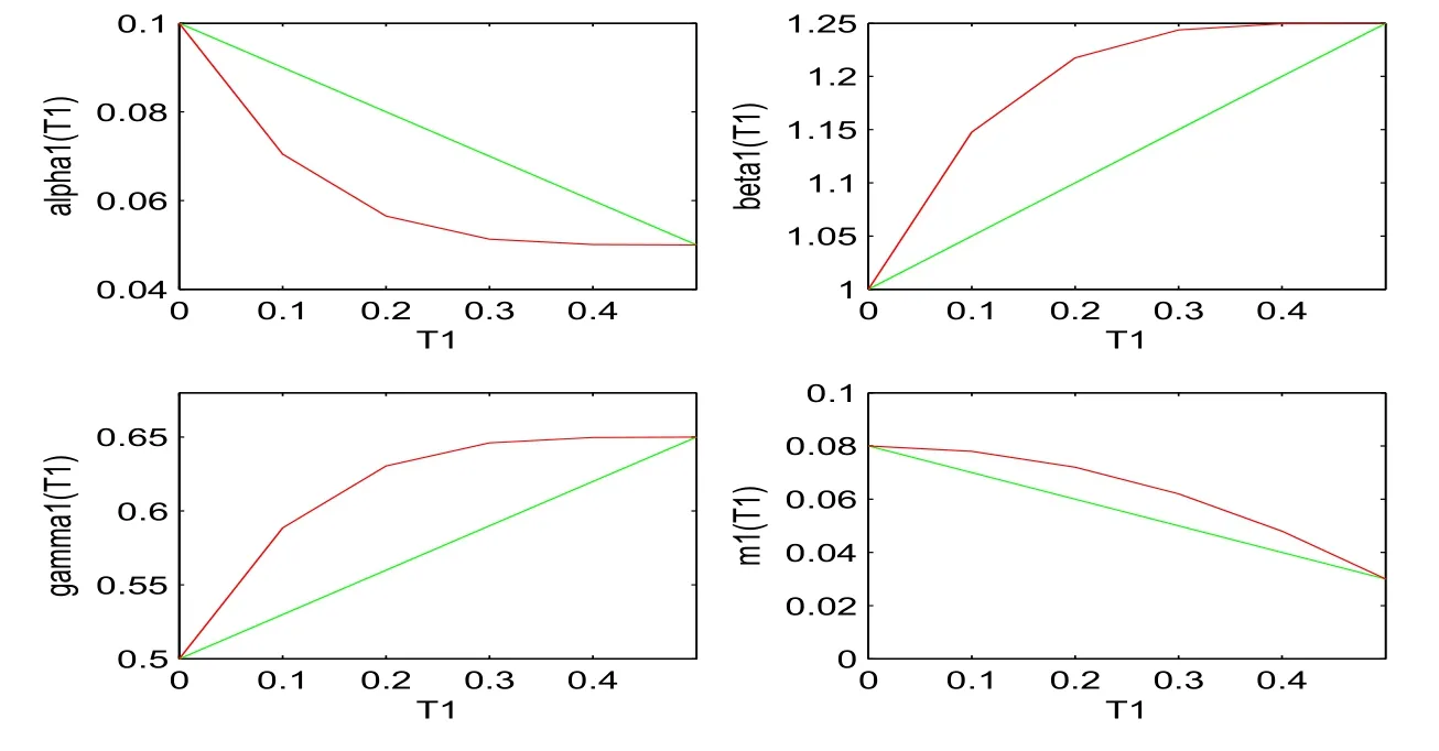
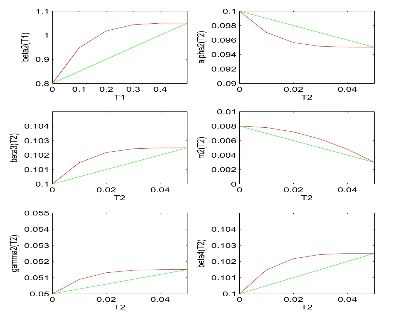
Figure 1: α1(T1), β1(T1), γ1(T1), m1(T1), β2(T1), α2(T2), β3(T2), m2(T2), γ2(T2)and β4(T2) are demonstrated from top to bottom respectively, where green lines denote the linear case (74) and red lines denote the nonlinear case (75).

Example 5.1We assume that the initial value of model (11) is (xi(0),xm(0),yi(0),ym(0),T1(0),T2(0)) = (0.5,0.5,0.8,0.8,0.01,0.001), and take parameters respectively are:α11= 0.25,α12= 0.1,β11= 1,β12= 0.5,γ11=γ12= 0.3,m11= 0.01,m12= 0.1,β21=β22= 0.5,α21=α22= 0.1,β31= 0.1,β32= 0.05,m21= 0.008,m22= 0.01,γ21= 0.05,γ22= 0.03,β41= 0.1,β42= 0.05,Q1= 0.4,Q2= 0.004,δ1=δ2= 0.8,δ3= 0.02,δ4= 0.002,δ5= 0.03,δ6= 0.003,E= 0.5,σ1=σ2=σ3=σ4= 0.3. It is easy to verify that conditions (28) of Theorem 3.1,(38) of Theorem 3.2, (43) of Theorem 3.3 and (44) of Theorem 3.4 are all satisfied respectively, then the extinction of model (11) is demonstrated in Figure 2.

Example 5.2Let parameters of model(11)beα11=1.1,α12=0.3,β11=0.35,β12=0.15,γ11=γ12=0.35,m11=m12=0.1,β21=0.045,β22=0.05,α21=1.05,α22= 0.1,β31= 0.2,β32= 0.1,m21= 0.4,m22= 0.15,γ21=γ22= 0.06,β41= 0.2,β42= 0.1,Q1= 0.3,Q2= 0.004,δ1=δ2= 0.8,δ3=δ4= 0.02,δ5=δ6= 0.03,E= 0.01,σ1= 0.1,σ2=σ3=σ4= 0.05. And, the initial value is (xi(0),xm(0),yi(0),ym(0),T1(0),T2(0))= (2,2,3,3,0.01,0.000 6). It is easy to verify that conditions (59) of Theorem 4.1, (63) of Theorem 4.2, (70) of Theorem 4.3 and (72) of Theorem 4.4 are all satisfied respectively, thenym(t) andxm(t) are strongly persistent in the mean,yi(t) andxi(t) are strongly persistent, which could be illustrated in Figure 3.

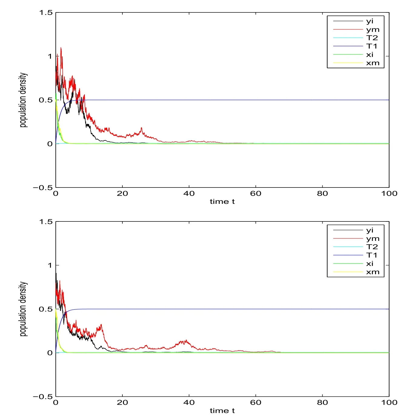
Figure 2: Extinction of xi(t), xm(t), yi(t) and ym(t) under linear case (top)and nonlinear case (bottom).

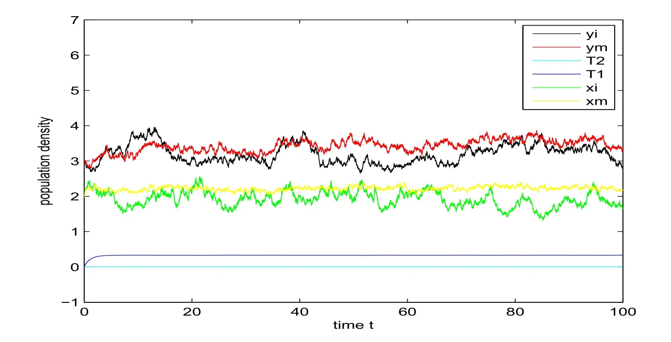
Figure 3: Strong persistence in the mean of ym(t) and xm(t), strong persistence for yi(t) and xi(t) under linear case (top) and nonlinear case (bottom).

6 Conclusion

In this paper,we propose a stochastic stage-structured single-species model with migrations and hunting within a pollution environment. The single-species moves between two patches: the unprotected and protected patch,and is separated into the immature and the mature, where the immature takes timeτto become the mature.

We show that model (11) admits a unique and global solution for any given initial value (12) by Lypapunov function method. We also obtain the main results of this paper by using the comparison theorem of stochastic differential equations,the strong law of large numbers and some inequalities.

Then the sufficient conditions guaranteeing the extinction of single-species are derived, which demonstrate that the population density of single-species depends on the birth/death rates. Meanwhile, the extinction of single-species also relies on the migration rates between the mature individuals in two patches as presented in Theorems 3.1 and 3.3. For the mature individuals in the unprotected patch, the population density is controlled by the hunting rate in Theorem 3.3.

We also derive the sufficient conditions for the persistence of single-species when the intensities of the white noises are bounded(see parameter-dependent conditions(59), (63), (70) and (72)). We find that the population density for the persistence with linear case is higher than that with nonlinear case as shown in Figure 3 (see the red lines).

We therefore would like to propose some possible strategies for single-species within two patches,for instance,setting obstacles on boundaries to maintain rational migration rates and enhancing punishment to decrease hunting rates. In practice,there are two possible options for deducing the toxicant concentration for singlespecies by use of some artificial methods: appropriately cutting down the pollutant outflow through closuring of the polluters and improving the afforestation within patches to single-species.