Stochastic Contrast Measures for SAR Data:A Survey

Alejandro C.Frery

Abstract:“Contrast”is an generic denomination for“difference”.Measures of contrast are a powerful tool in image processing and analysis,e.g.,in denoising,edge detection,segmentation,classification,parameter estimation,change detection,and feature selection.We present a survey on techniques that aim at measuring the contrast between (i)samples of SAR imagery,and (ii)samples and models,with emphasis on those that employ the statistical properties of the data.

Key words:Contrast;Divergence;Entropy;Geodesic distance;Statistics;Synthetic Aperture Radar (SAR)

1 Introduction

Synthetic Aperture Radar (SAR)has been widely used as an important system for information extraction in remote sensing applications.Such microwave active sensors have as main advantages the following features:(i)their operation does not depend on sunlight,either of weather conditions and (ii)they are capable of providing high spatial image resolution.

In recent years,the interest in understanding such type of imagery has increased.However,since the acquired images stem from a coherent illumination process,they are affected by a signaldependent granular noise called“speckle”[1].Such noise has a multiplicative nature,and its intensity does not follow the Gaussian law.Moreover,the availability of fully polarimetric images requires processing data in the form of complex matrices.Thus,analyzing SAR images requires tailored image processing based on the statistical properties of speckled data.

There is a vast literature on techniques for SAR image processing and analysis that employ a diversity of approaches for the related problems these images pose.Among them,advances in modeling with Statistical Information Theory and Geometry have led to several exciting solutions for the problems of denoising,edge detection,segmentation,classification,parameter estimation,change detection,and feature selection.Moreover,these approaches provide unique insights on the properties of the data and the information they convey.

This paper presents a survey of those results.

This work is organized in nine sections following this Introduction.

Section 2,where we show that it is possible to assess the quality of despeckling filters by measuring the distance of the denoised image to the ideal model.

Once we see that the approach provides interesting results,we move to Section 3,where we review the main inference techniques,namely analogy(Sec.3.1),maximum likelihood (Sec.3.2),and Nonparametric and Robust estimation (Sec.3.3).

Section 4 discusses the main approaches for computing differences between distributions:the logarithm of the ratio of likelihoods (Sec.4.1),tests based on divergences (Sec.4.2),tests that rely on the quadratic difference of entropies (Sec.4.3),and tests that employ geodesic distances between distributions (Sec.4.4).

Section 5 reviews the main models that describe SAR data in intensity format,and provides details about the Gamma (Sec.5.1)andG0(Sec.5.2)distributions.

Section 6 presents applications of the concepts discussed in Section 4 to the intensity models of the previous one:edge detection by maximum likelihood (Sec.6.2)and by maximum geodesic distance between samples (Sec.6.3);parameter estimation by distance minimization (Sec.6.4);and speckle reduction (Sec.6.5).

Section 7 reviews the main distribution for fully polarimetric data:the Wishart law.We present the reduced log-likelihood of a sample from such a model and estimation by maximum likelihood.

In Section 8,we study applications of measures of difference to polarimetric data:we propose a nonlocal filter whose weights are proportional to the closeness between samples (Sec.8.1);we classify segments by minimizing the distance between samples and prototypes (Sec.8.2);we go back to the problem of edge detection in this kind of data (Sec.8.3);we show a technique for polarimetric decomposition,which corrects the effects of the orientation angle (Sec.8.4),and we conclude showing how to detect changes in multitemporal images with a test based on likelihoods and by comparing entropies (Sec.8.5).

Section 9 presents the idea of projecting polarimetric data onto the surface of a 16-dimensional sphere,measuring distances and,with this,performing decompositions and clustering.

Fig.1 shows the mind map that led the writing of this survey.The arrows denote the model and/or technique used to tackle each problem.

The paper concludes with Section 10,where we suggest research avenues and further readings.We also give our assessment of the value of these techniques in perspective in an era dominated by the Deep Learning approach.

2 Filter Assessment

The multiplicative model is widely accepted as a good descriptor for SAR data[2].It assumes that the observed intensityZin each pixel is the product of two independent random variables:X,which describes the unobserved backscatter (the quantity of interest),andY,the speckle.

One can safely assume that the speckle obeys a Gamma law with unitary mean and shape parameterL,the number of looks,which depends on the processing level and is related to the signal-tonoise ratio.

Without making any assumption about the distribution ofX,except that it has positive support,any despeckling filtermay be seen as an estimator ofXbased solely on the observation of.Argentiet al.[3]present a comprehensive survey of such filters,along with measures of their performance.

Fig.1 Mind map of this review contents

Image processing platforms suited for SAR,e.g.,ENVI1https://www.harrisgeospatial.com/Software-Technology/ENVI/and Snap2https://step.esa.int/main/toolboxes/snap/,offer users a plethora of despeckling filters,and all of them require stipulating parameters.The final user seldom chooses measures of quality,as they capture different features,and there is no obvious way to combine them.

Gomezet al.[4]noted that the ideal filtershould produce the actual backscatterXas output.The ideal ratio imageis a collection of independent identically distributed (iid)Gamma deviates with unitary mean and shape parameterL.The worse the filteris,the further (less adherent)the ratio imagewill be from this model.They then proposed measuring this distance with two components:one,based on first-order statistics(mean and looks preservation),and the other based on second-order statistics (how independent the observations are).This distance can also be used to fine-tune the parameters of a filter in order to obtain optimized results.

The first component is comprised of quadratic differences between (i)local means that should be 1 and (ii)local estimates of the shape of the Gamma distribution that should be equal to the original number of looks.

The second component was initially measured through the homogeneity from Haralik’s cooccurrence matrices[5].The original proposal used as reference an ensemble of shuffled ratio images.Vitaleet al.[6]improved this step by comparing the joint and marginal distributions of the co-occurrence matrices.

Later,Gomezet al.[7]studied the statistical properties of this measure,leading to a test whose null hypothesis is that the filter is ideal.This approach led to a powerful tool without assuming any distribution forX,thus forZ.

However,we need potent models in order to extract information from SAR images.These models will be reviewed in Sections 5 and 7.

3 Statistical Inference

This Section is based on the book by Frery and Wu[8],freely available with code and data.

Assume we have data and models for them.We will see ways of using the former to make inferences about the latter.

Without loss of generality,consider the parametric model (Ω,A,Pr)for real independent random variablesXandX=(X1,X2,...),in whichΩis the sample space,Ais the smallestσ-algebra of events,and Pr is a probability measure defined onA.The distribution ofXis indexed bywherep ≥1 is the dimension of the parametric space

Parametric statistical inferences consist in making assertions aboutθusing the information provided by the sampleX.

3.1 Inference by analogy

This approach requires the knowledge of the expected value of transformations of the random variableX:

where eachψjis a measurable functionEach element of Eq.(1)is given by

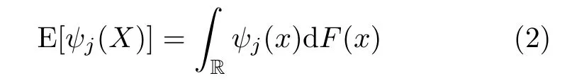
andFis the cumulative distribution function ofX.Ifψ(X)=Xk,we say that E (Xk)is thek-th order moment ofX(if it exists).

The quantity E(X -EX)kis called“the central moment”ofX,if it exists.The second central momentis called“the variance”ofX.We denote it Var(X).

The Law of Large Numbers is the basis for inference by analogy[9].This law states that (under relatively mild conditions)holds that

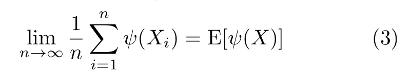
providedX,X1,X2,...are iid.

With this in mind,and assuming one has a large sample,it seems reasonable to equate sample quantities (the left-hand side)and parametric expressions (the right-hand side).

When we havepparameters,i.e.we needplinearly independent equations to form an estimator ofθ.Such estimator has the following form:

More often than not,one has to rely on numerical routines to obtainwith this approach.In some cases,Eq.(4)has no solution;cf.[10].

3.2 Inference by maximum likelihood

Consider again the sample of iid random variableseach with the same distribution characterized (without lack of generality)by the density.The likelihood function is

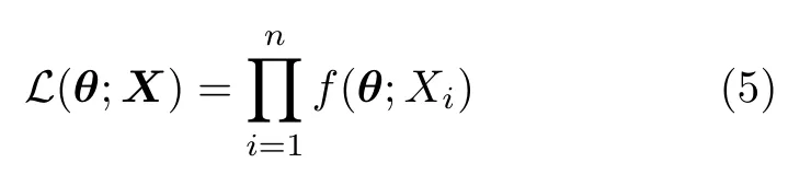
Notice thatis not a joint density function,as it depends onθ,not on the variables.

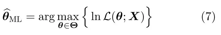
The principle of maximum likelihood proposes as estimator forθthe parameter that maximizes Eq.(5):

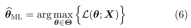
that is,the point inΘthat makes the observ ations most plausible.It sometimes coincides with some analogy estimators.

The two most widely used approaches for maximizing Eq.(5)are by optimization and by the solution of a system of equations.They both operate on the reduced log-likelihood rather than on Eq.(5).

Using the fact that Eq.(5)is a product of positive functions,one may consider

instead of Eq.(6).If we now discard from lnthe terms that do not depend onθ,we obtain the reduced log-likelihoodour function of interest.

A maximum likelihood estimator may be found by maximizingoften with numerical tools,or by solving the system of equations given by

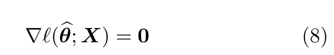
i.e.,the partial derivatives with respect to eachθiequated to zero.

Both approaches often require an initial solution,and a general recommendation is towards using an analogy estimator (if available)for that purpose.

Provided there are no doubts about the validity of the model,the maximum likelihood estimators should be preferred over those obtained by analogy.

3.3 Other inference techniques

There are two remarkable approaches to statistical inference that differ from analogy and maximum likelihood:nonparametric and robust estimation.

The nonparametric approach makes little or no assumptions about the underlying distribution of the data.Cintraet al.[11]employed such techniques with success for the problem of finding edges in SAR imagery.Nonparametric estimators are resistant to contamination,at the expense of having less efficiency.They should be part of every practitioner’s toolbox.The interested reader is referred to the books listed in Refs.[12-14]for details about this approach.

The reader must always bear in mind the underlying hypotheses used to devise an inference procedure.All the techniques discussed above assume that the sample is comprised of observations from iid random variables.A middle path between parametric (Analogy and maximum likelihood)and nonparametric is the robust approach.

Robust inference assumes there is a model of interestD(θ), and that we aim at estimatingθwith a sampleZ=(Z1,Z2,...,Zn).The sample may or may not be produced byD(θ)as hypothesized.

A robust estimator forθshould behave well when the model is correct,although notasgood as the maximum likelihood estimator(by definition).However,differently fromit should provide acceptable estimates whenZoriginates from a different distribution,i.e.,under the presence of contamination.

Contamination may describe several departures from the primary hypothesis as,for instance,a few gross errors when registering the observations,or the presence of data originated from a different law.Contamination happens,for instance,when computing local statistics for designing a filter.The underlying assumption thatZconsists of observations from iid random variables breaks when the estimation window is transitioning over two or more different areas.The works by Palacioet al.[15]and by Negriet al.[16]examine the impact that mild violations of this hypothesis on the behavior of subsequent operations,when the inference procedure is unaware of such departure.

Freryet al.[17]proposed robust estimators for speckle reduction in single-look amplitude data.The authors used an empirical approach and devised estimators based on trimmed statistics,on the median absolute deviation,on the inter-quartile range,on the median,and on the best linear unbiased estimator.They compared the performance of these techniques with respect to estimators based on analogy (moments)and maximum likelihood and concluded that it is advisable to consider robust procedures.

More recently,Chanet al.[18]used a connection between the model defined by (21)and the Pareto distribution to propose robust estimators with low computational cost.The authors show applications to region classification in the presence of extreme values caused by,for instance,corner reflectors.

Refs.[19-21]discuss other robust techniques for inference with small samples under contamination.

The visible gain in using robust estimators in speckle reduction techniques is a reduced blurring of the edges and the preservation of small details in the image.This advantage usually comes at the cost of more computational resources.

4 Measures of Difference

Several relevant problems in signal and image processing and analysis can be solved by formulating them in the form of the following hypothesis test:

Consider theN ≥2 samplesz1,z2,...,zNof the formzj=z1,j,z2,j,...,znj,jfor every 1≤j ≤N.Is there enough evidence to reject the null hypothesis that they were produced by the same model

This problem assumes that theNsamples might be of different sizesn1,n2,...,nN,and that the modelD(θ)is a probability distribution indexed by the unknownq-dimensional parameterEventually,there might be no known model,and it will have to be learned from the data and the underlying hypotheses of the problem.

In most of this review,with the exception of Section 4.3,we will be handling two samplesz1,z2of sizesn1andn2of the formand

In the following,we will review some of the relevant approaches in the context of SAR image analysis,which have proven to be relevant at handling this problem.

4.1 Likelihoods ratio

The ratio of likelihoods (LR)statistic is of great importance in inference on parametric models.It is based on comparing two (reduced)likelihoods utilizing a ratio of two maxima:the numerator is the likelihood in the alternative hypothesis,and the denominator is the likelihood in the null hypothesis.These hypotheses must be a partition of the parametric space:.Under the null hypothesis,the denominator of the test statistic should be large compared to the numerator yielding a small value.

As discussed in Ref.[22],such statistic has,underan asymptotic distribution,whereqis the difference between the dimensions of the parameter spaces under the alternative and the null hypotheses.It is,thus,possible to obtainpvalues.

4.2 Tests based on divergences

This section is based on the work by Nascimentoet al.[23].Contrast analysis requires quantifying how distinguishable two samples are requiring.Within a statistical framework,this amo unts to providing a test statistic for the null hypothesis that the same distribution produced the samplesthe parameter space.

Information theoretical tools collectively known as divergence measures,offer entropybased methods to discriminate stochastic distributions[24]statistically.Divergence measures were submitted to a systematic and comprehensi ve treatment in Refs.[25-27]and,as a result,the class of (h,ϕ)-divergences was proposed[27].

LetXandYbe random variables defined over the same probability space,equipped with densitiesrespectively,whereθ1andθ2are parameter vectors.Assuming that both densities share a common supportI ⊂ℝ,the (h,ϕ)-divergence betweenfXandfYis defined by

whereϕ:(0,∞)→[0,∞)is a convex function,h:(0,∞)→[0,∞)is a strictly increasing function withh(0)=0,and indeterminate forms are assigned value zero.

By a judicious choice of functionshandϕ,some well-known divergence measures arise.Tab.1 shows a selection of functionshandϕthat lead to well-known distance measures.Specifically,the following measures were examined:(i)the Kullback-Leibler divergence[28],(ii)the relative Rényi (also known as Chernoff)divergence of orderβ[29,30],(iii)the Hellinger distance[31],(iv)the Bhattacharyya distance,(v)the relative Jensen-Shannon divergence[32],(vi)the relative arithmetic-geometric divergence,(vii)the triangular distance,and (viii)the harmonic-mean distance.

Often not rigorously a metric[33],since the triangle inequality does not necessarily hold,divergence measures are mathematically suitable tools in the context of comparing distributions.Additionally,some of the divergence measures lack symmetry property.Although there are numerous methods to address the symmetry problem[34],a simple solution is to define a new measuregiven by

(i)The Kullback-Leibler distance:

(ii)The Rényi distance of orderβ:

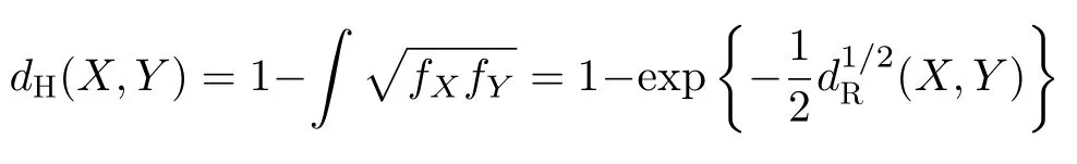
(iii)The Hellinger distance:

(iv)The Bhattacharyya distance:

(v)The Jensen-Shannon distance:

(vi)The arithmetic-geometric distance:

Tab.1 (h,ϕ)-divergences and related functions ϕ and h

(vii)The triangular distance:

(viii)The harmonic-mean distance:

We conclude this section stating one of the basilar results that support all the forthcoming techniques.

The distances mentioned above are neither comparable nor semantically rich.Refs.[35-37]are pioneering works that make a connection between anyh-ϕdistance and a test statistic.

Consider the modelD(θ), withan the unknown parameter that indexes the distribution.Assume the availability of two samples of iid observationsfromandfromCompute the maximum likelihood estimators ofθ1andWe are interested in verifying if there is enough evidence into reject the null hypothesis

Under the regularity conditions discussed in Ref.[27,p.380]the following lemma holds:

Lemma 1:Ifn1/(n1+n2)converges to a constant in (0,1)whenn1,n2→∞, andθ1=θ2,then

Based on Lemma 1,we obtain a tests for the null hypothesisθ1=θ2in the form of following proposition.

Proposition 1:Letn1andn2be large andthen the null hypothesisθ1=θ2can be rejected at levelαif

This result holds for everyh-ϕdivergence,hence its generality.The (asymptotic)p-value of thestatistic can be used as a measure of the evidence in favor ofH0,so it has rich semantic information.As the convergence is towards the same distribution,these values are comparable.

4.3 Tests based on the quadratic difference of entropies

The test statistic presented in Section 4.2 comparesapair ofmaximumlikelihoodestimatorsMany applications,as,forinstance,change detection in time series,requires using more evidence.In such cases it is possible to compare entropies.

For such situations,one may rely on tests based on entropies,as described in the following results,which are based on Ref.[38].

Letf(z;θ)be a probability density function with parameter vectorθ.Theh-ϕentropy relative toZis defined by

where eitherϕ:is concave andh:is increasing,orϕis convex andhis decreasing.Tab.2 shows the specification of five of these entropies:Shannon,Rényi,Arimoto,Sharma-Mittal,and restricted Tsallis.

The following result,derived by Pardoet al.[37],paves the way for the proposal of asymptotic statistical inference methods based on entropy.

Lemma 2:Letbe the ML estimate of the parameter vectorθof dimensionMbased on a random sample of sizenunder the modelf(z;θ).Then

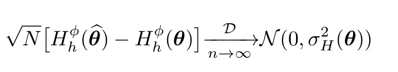
whereN(µ,σ2)is the Gaussian distribution with meanµand varianceσ2,

K(θ)=E{-∂2lnf(z;θ)/∂θ2}is the Fisher information matrix,andδ=[δ1δ2...δp]Tsuch that

We are interested in testing the following hypotheses:

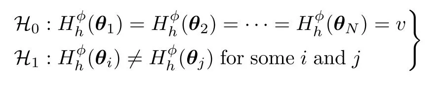
In other words,we seek for statistical evidence for assessing whether at least one of theNsamples has different entropy when compared to the remaining ones.

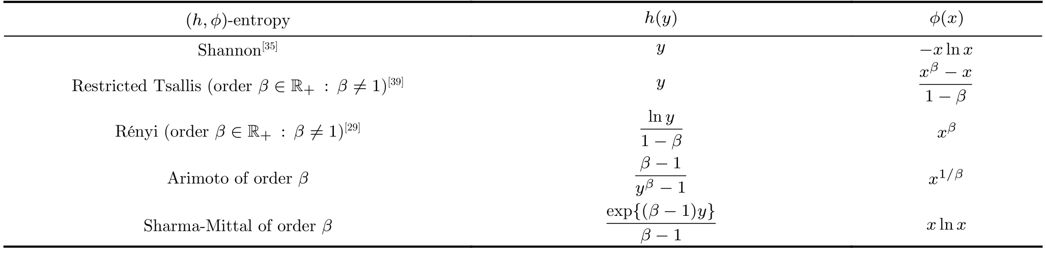
Tab.2 h-ϕ entropies and related functions

fori=1,2,...,N.Therefore,

Sincevis,in practice,unknown,in the fol lowing we modify this test statistic in order to take this into account.We obtain:

where

Salicrúet al.[35]showed that the second summation in the right-hand side of Eq.(14)is chisquare distributed with one degree of freedom.Since the left-hand side of Eq.(14)is chi-square distributed withNdegrees of freedom (cf.Eq.(13)),we conclude that:

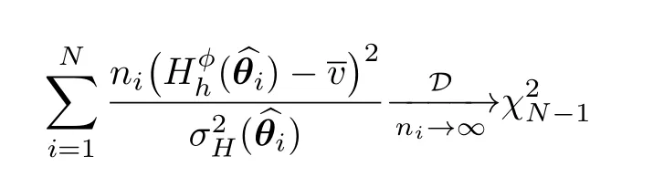
In particular,consider the following test statistic:

We are now in the position to state the following result.

Proposition 2:Let each sample sizeni,i=1,2,...,N,be sufficiently large.Ifs,then the null hypothesiscan be rejected at a levelαif

Again,this Proposition transforms a mere distance into a quantity with concrete meaning:apvalue.

4.4 Tests based on geodesic distances

Assume we are characterizing the data by the distribution,so each population is completely described by a particular pointThe information matrix of the model has entries

According to Ref.[40],it can be used to measure the variance of the relative difference between two close models as

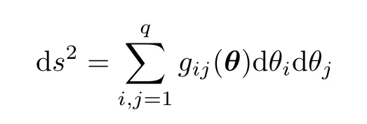
This quadratic differential form is the basis for computing distances between models with

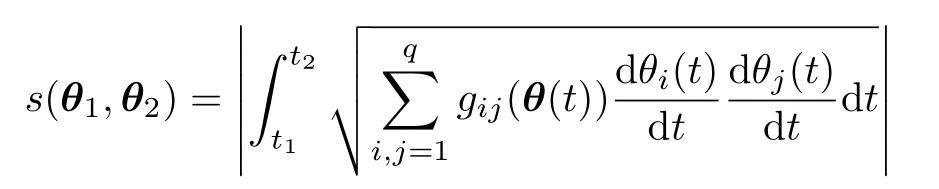
whereθ(t)is a curve joiningθ1andθ2such thatθ(t1)=θ1andθ(t2)=θ2.Among all possible curves,we are interested in the shortest one;this leads to the geodesic distance between the models.Finding such a curve is,in general,very difficult,in particular,for distributions with parameters other thanq=1.

An alternative approach consists in considering distribution families with a scalar parameterwithq=1.With this restriction in mind,we can define a generalized form of distance:that based onh-ϕentropies as the solution of

where

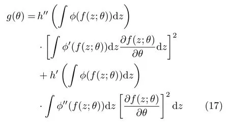
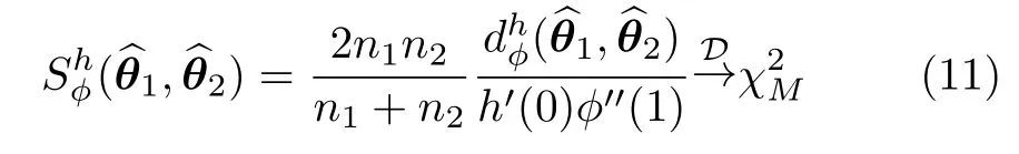
In analogy with the results presented for entropies and divergences,Menéndezet al.[41]proved the following asymptotic result:consider,for simplicity,h(y)=yandϕas in previous sections.The test statistic

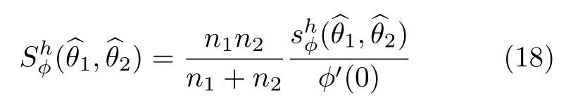
has,under the nullhypothesisθ1=θ2and for sufficiently largen1andn2,asymptotic distribution.

The classical geodesic distance is obtained whenhandϕare those leading to the Shannon entropy;cf.Tab.2.In this case,g(θ)becomesg11(θ),the only element of Eq.(16).

This alternative approach is more tractable,but requires a further step,namely joining theqtest statistics into a single measure of dissimilarity.After Naranjo-Torreset al.[42]showed the ability of the Shannon geodesic distance at finding edges in intensity SAR data,Frery and Gambini[43]compared three fusion techniques.

5 Intensity Data

The most famous models for intensity SAR data are the Gamma,K,andG0distributions.Ref.[44]presents a survey of models for SAR data.The first is adequate for fully developed speckle,while the two others can describe the texture,i.e.,variations of the backscatter between pixels with an additional parameter.Their probability density functions are,respectively:

where,in Eq.(19)µ＞0 is the mean;in Eq.(20)λ,α ＞0 are the scale and the texture,andKνis a modified Bessel function of orderν;and in Eq.(21)γ ＞0 is the scale andα＜0 is the texture.In all these expressions,L ≥1 is the number of looks.

Maximum likelihood estimators require iterative methods that may not converge,and estimators by analogy may not have feasible solutions.Moreover,contamination is a significant issue,mostly when dealing with small samples and/or in the presence of strong backscatter as the one produced by a double bounce.

The models given by Eq.(19)and Eq.(21)are basilar to this work.The next subsections present properties that will be useful in the sequence.

5.1 The Gamma model

The Gamma model given by Eq.(19)includes the Exponential distribution whenL=1,i.e.,in the single-look case.Fig.2 shows the densities that characterize this distribution with varying means.The linear scale (Fig.2(a))shows the well-known exponential decay,while in the semilogarithmic scale (Fig.2(b))they appear as straight lines with a negative slope.

Fig.3 shows the effect of multilooking the data on their distribution:it shows three densities with the same mean (µ=1)andL=1,3,8.The largerLbecomes,the smaller the probability of extreme events,as can be seen in the semilogarithmic scale (Fig.3(b)).Also,asLincreases,the densities become more symmetric;cf.Fig.3(a).

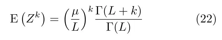
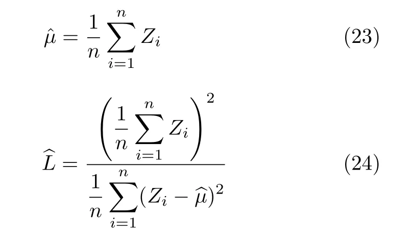
Assume one has a sample ofniid Γ (µ,L)deviatesZ=(Z1,Z2,...,Zn).Inference about (µ,L)can be made by the analogy method using the moments given in Eq.(22).For instance,choosing to work with the first moment and the variance,one has:i.e.,the sample mean and the square of the reciprocal sample coefficient of variation.

Usually,one selects samples from areas where the Gamma model provides a good fit and estimates the number of looks which,then,is employed for the whole image.

As an alternative to any analogy method,one may rely on maximum likelihood estimation.From Eq.(19),one has that the reduced loglikelihood of the sampleZis

The maximum likelihood estimator of (µ,L)is the maximum of Eq.(25).This maximum may be found by optimization of Eq.(25),or by solving the system of equations given by

This second approach to obtaining the maximum likelihood estimator of (µ,L)leads to Eq.(23)and to the solution of

Fig.2 Exponential densities with mean 1/2,1,and 2 (red,black and blue,resp.)in linear and semilogarithmic scales

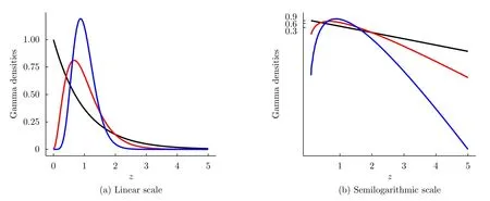
Fig.3 Unitary mean Gamma densities with 1,3,and 8 looks (black,red,and blue,resp.)in linear and semilogarithmic scales

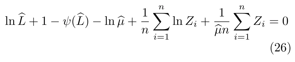
whereψis the digamma function.

Either way,optimization or finding the roots of Eq.(26),one relies on numerical procedures that,more often than not,require a starting point or initial solution.Moment estimators are convenient initial solutions for this.

5.2 The model

Freryet al.[45]noticed that theKdistribution failed at describing data from extremely textured areas as,for instance,urban targets.The authors then proposed a different model for the backscatterX:the Reciprocal Gamma distribution.

forx ＞0 and zero otherwise.

Now introducing the Reciprocal Gamma model for the backscatter in the multiplicative model,i.e.by multiplying the independent random variablesX～Γ-1(α,γ)andY～Γ(1,L),one obtains thedistribution for the returnZ=XY,which is characterized by the density Eq.(21).It is noteworthy that,differently from Eq.(20),this density does not involve Bessel functions.

We denote(α,γ,L)the situation ofZfollowing the distribution characterized by Eq.(21).Thek-order moments ofZare

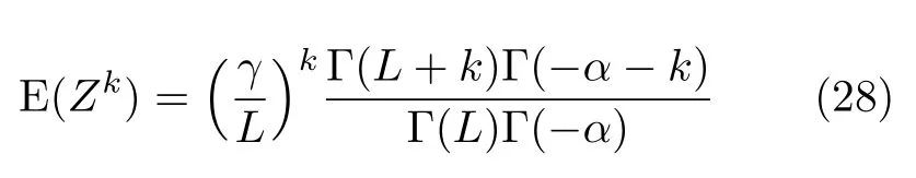
provided-α＞k,and infinite otherwise.Eq.(28)is useful,among other applications,for findingγ∗=-α-1,the scale parameter that yields a unitary mean distribution for eachαand anyL.It also allows forming systems of equations for estimating the parameters by analogy.

Fig.5 shows the effect of varying the number of looks,for the sameα=5 andγ=4.

Notice,again,in Fig.5(b)the effect multilook processing has mostly on the distribution of minimal values.Such effect,along with the reduced probability of huge values,have with multilook processing,yields less contrasted images.

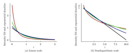
Fig.4 Densities in linear and semi-logarithmic scale of the E (1)(black)and distributions with unitary mean and α ∈{-1.5,-3.0,-8.0} in red,green,and blue,resp

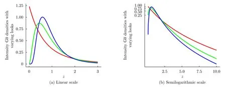
Fig.5 Densities in linear and semilogarithmic scale (-5,4,L)distributions with unitary mean and L ∈{1,3,8} in red,green,and blue,resp

The distribution relates to the well-known Fisher-Snedekor law in the following manner:

where Υu,vis the cumulative distribution function of a Fisher-Snedekor distribution withuandvdegrees of freedom,andis the cumulative distribution function of arandom variable.Notice that Υ is readily available in most software platforms for statistical computing.Since such platforms usually also provide implementations of the inverse of cumulative distribution functions,the Inversion Theorem can be used to sample from thelaw.

Assume that we have a sampleof iid random variables that follow thedistribution,i.e.,Lhas been already estimated by.The unknown parameter

The maximum likelihood estimator of (α,γ),is any point that maximizes the reduced log-likelihood:

provided it lies inΘ.Maximizing Eq.(30)might be a difficult task,in particular in textureless areas whereα→-∞and thedistribution becomes very close to a Gamma law.

6 Applications to Intensity Data

6.1 Estimation of the equivalent number of looks

The three models for intensity data presented in Eqs.(19)-(21)have one parameter in common:L,the number of looks.Such feature is absent in empirical models[44],and describes the number of independent samples used to form the observationZat each pixel.It is a direct measure of the signal-to-noise ratio and,thus,of the visual quality of the image.

Although it is usually part of the image information,such nominal value is often larger than the evidence provided by the data.It is,thus,important to estimate this quantity in order to make a fair statistical description of the observations.

Fig.6 shows a 400×1000 pixels intensity image obtained by the ESAR sensor[47]sensor in Lband and VV polarization.The area consists of agricultural parcels,a river (the dark curvilinear feature to the right),and a bright urban area to the lower right.The data have been equalized for visualization purposes,and we also show a regular grid comprised of squares of 25×25 pixels that aids obtaining disjoint samples.

Fig.6 Equalized intensity data with grid

Assume we have collectedNsamplesz1,z2,...,zNof the formfor every 1≤j ≤Nfrom areas which do not exhibit any evidence of not belonging to the Gamma distribution (at least,they do not show texture).These samples might be of different sizesn1,n2,...,nN.Among the many possible approaches for estimating the number of looks,we will consider two of the simplest and most widely used in the literature.In both cases,we will assume that aΓ(µj,L)model holds for all the samples,i.e.,that the mean may vary but not the number of looks.

In general,it is preferred to take several small disjoint samples with some spatial separation.This alleviates the problem of using correlated rather than independent observations.

The forthcoming results were obtained withN=12 samples of equal sizen=625 each.

(1)Weighted mean of estimates:Use each sample in Eqs.(23)and (24)to obtain theNestimatesthen compute the final estimate by the weighted average

With the data collected over the image shown in Fig.6 we obtained

(2)Regression:From Eq.(22)we have that Var(Z)=µ2/L,then the coefficient of variationWith this,we may form the equation

We nowcomputethe sample meanand vari anceof eachsamplezj,and form thefollowing regression model data:

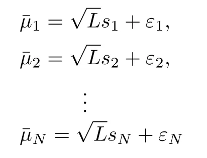
Notice that,although equivalent,we preferred to denote the sample mean asinstead ofto elucidate the difference between simple mean and parameter estimation.Assuming further that the errorsare iid zero mean Gaussian random variables with unknown variance,we are now in position to apply a simple regression model without intercept to estimateL.

Denote the dependent variablethe independent variables=(s1,s2,...,sN)T, and the errorsε=(ε1,ε2,...,εN)T,where the superscript“ T”denotes the transpose.The model isand the estimate ofLby regression is then given by

Since the equivalent number of looks is assumed,in many cases,constant over the whole image,it is of paramount importance to make a careful estimation.

In the two following sections,the notion of“contrast”is the difference of statistical properties between two samples.

6.2 Edge detection by maximum likelihood

Besides providing estimators with excellent properties,the likelihood function can also be used to find edges.The approach proposed in Refs.[48-50]consists in forming a likelihood that models a strip of data,and finding the point where it is maximized.This point will,then,be the estimator of the edge position.

Fig.8 illustrates the rationale behind this proposal.It shows strips of 10×500 pixels with samples from twodistributions:(-1.5,0.5,3.0)in the left half,and(α2,-α2-1,3)in the right half,withα2∈{-20,-10,-5,-3}.The two halvesseemdistinguishable after image equalization in the first three cases,but the reader must notice that they have the same unitary mean.With this,techniques that rely on the classical notion of contrast are doomed to failure.

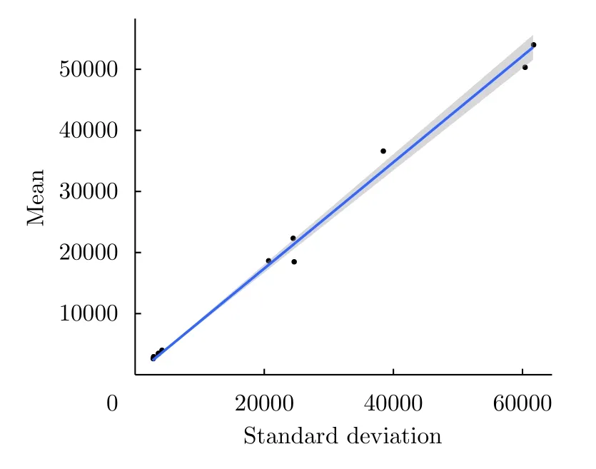
Fig.7 Regression analysis for the estimation of the equivalent number of looks

Instead of relying on the mean,the Gambini Algorithm aims at finding the point where the total log-likelihood of the samples is maximum.It is sketched in Algorithm 1.

Algorithm 1:The Gambini Algorithm for edge detection using maximum likelihood

Fig.9 shows three total log-likelihoods.The bigger the difference between the parameters is,the more pronounced the maximum is.Notice that all the maxima are close to the correct edge position,which is located atj=250.The two pronounced local minima are due to the lack of convergence of the optimization algorithm.

This approach and the likelihoods ratio are closely related,with the former being the denominator of a test statistic of the latter.

It is noteworthy that the Gambini Algorithm is flexible,as it allows using any measure in place of the total log-likelihood function.

6.3 Edge detection by distance maximization

The previous approach at edge detection maximizes the total likelihood of the two strips.In this sense,the total log-likelihood is the function to be optimized.

Another approach consists in maximizing a distance between the models to the right and to the left of the moving point.The rationale is the same as before:the models will be maximally different when the samples are not mixed,i.e.,at the point which separates them into two different parts.

Algorithm 2 sketches an implementation of this approach.

Algorithm 2:The Gambini Algorithm for edge detection using a distance between models

Algorithm 2:The Gambini Algorithm for edge detection using a distance between models

The following points are noteworthy in Algorithm 2:

• The sampleszLandzRonly enter once,when computing the estimatesrespectively.This leads to faster algorithms than those based on the total log-likelihood,which use the sample twice.

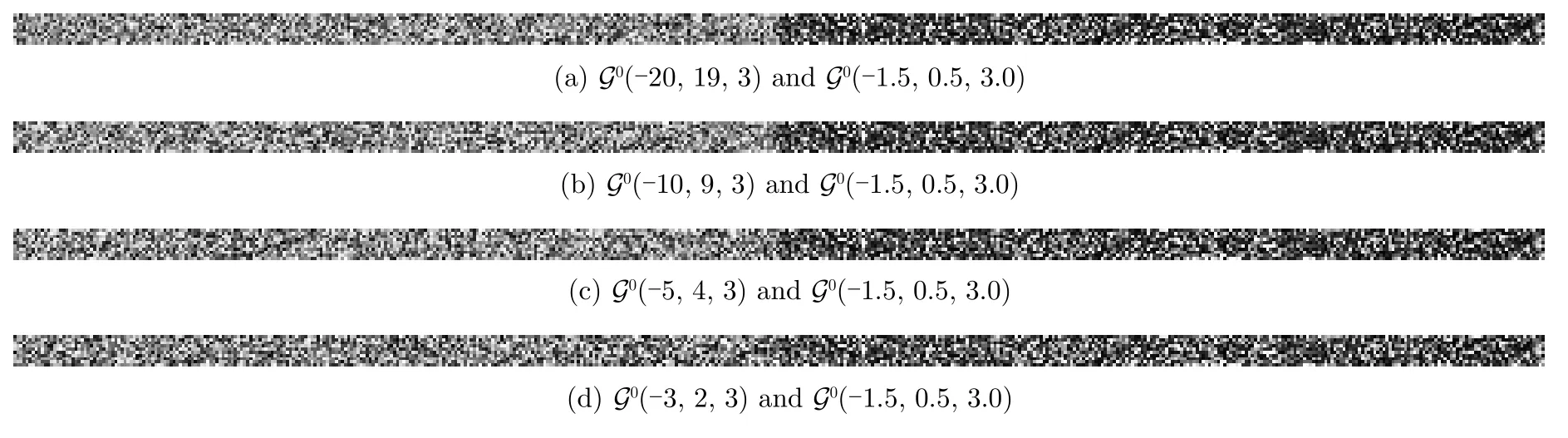
Fig.8 Strips of 10 × 500 pixels with samples from two distributions

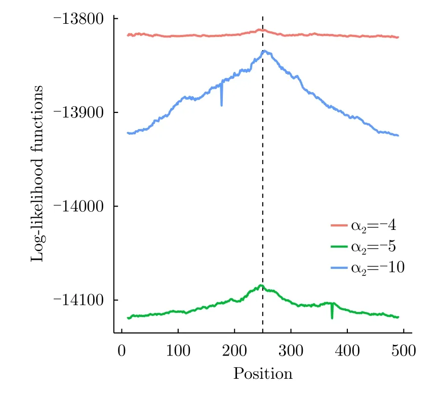
Fig.9 Illustration of edge detection by maximum likelihood

• If the distancesbelongs to either the class ofh-ϕdivergences or geodesic distances can be turned into a test statistic.With this,there is an important additional piece of information:the answer to the question,“Is there enough evidence to considerj⋆an edge?”

• Again,any model is suitable for this approach.

Naranjo-Torreset al.[42]used the Shannon geodesic distance,obtaining remarkable results.They also used this distance to measure the separability of classes.

6.4 Parameter estimation by distance minimization

In this section,“contrast”is the lack of adequacy of the model with respect to the observed data.

Nascimentoet al.[23]computed several of the distances and statistical tests presented in Sec.4.2 Being the null hypothesis that two samples come from the samelaw,they used these statistics as contrast measures.

Theh-ϕfamily of statistical tests is not the only way to measure the difference between samples.Still under themodel,Naranjo-Torreset al.[42]computed the Shannon Geodesic distance and,using results from Ref.[41]derived another class of tests useful for edge detection.Frery and Gambini advanced these results[43],proposing tests based on the composition of marginal evidence.These tests proved their usefulness in the detection of edges,even in situations of very low contrast.

Noting that the histogram is a stable density estimator,Gambiniet al.[51]proposed an estimation technique which consists in minimizing a distance between thedensity and a smoothed version of the histogram.The authors analyzed several smoothing techniques and distances obtained from the symmetrization ofh-ϕdivergences.The proposal consists of using kernel smoothing,and the triangular distance.

Fig.10 illustrates the procedure.The density that characterizes the modelis shown in light blue,along with the histogram of a sample of size 500 fromZ.The two black densities are the starting point (dashed line),and an intermediate step.The final estimate is the density in red.

Notice that this procedure may be used with any model.

6.5 Speckle reduction by nonlocal means

In this section,the“contrast”is inversely proportional to the similarity between two samples.

The Nonlocal Means approach is a new way of handling noise reduction[52,53].The idea is forming a large convolution mask that,differently from the classical location-invariant approach,is computed for every pixel to be filtered.The weight at position (k,ℓ)is proportional to a measure of similarity between the observationzk,ℓandzi,j,the pixel to be filtered.Such similarity is usually computed using the information in surrounding estimation windows (patches)∂k,ℓand∂i,jaround the pixels.The procedure typically spans a large (search)window,much larger than in typical applications.

Fig.10 Illustration of parameter estimation by distance minimization

Fig.11 illustrates this idea with a search window of size 9×9 around the central pixelzi,j,and patches of size 3×3.

The central weight of the convolution mask,wi,jis set to 1.The weightwk,ℓwill be a measure of the similarity between the values aroundzk,ℓandzi,j,highlighted with dark lines.Such similarity may be computed directly between the observations,or between descriptors of each patch:

Teuber and Lang[54]studied the properties of weights designed for the multiplicative model and how they behave in the presence of additive noise.Penna and Mascarenhas[55]included a Haar decomposition of the weights.

Ferraioliet al.[56]took a different approach.Instead of measuring the distance between the patches samples,they assumed a Square-Root-of-Gamma distribution for the data.IfZfollows aΓ distribution as in Eq.(19),thenZ1/2is Square-Root-of-Gamma distributed.Furthermore,the ratio of two independent of such random variables follows an Amplitudedistribution.Using this property,the authors checked how pertinent is the hypothesis that the two samples belong to the same distribution and used this information to compute the weights.

Fig.11 Illustration of the Nonlocal Means approach

The Nonlocal Means approach is flexible enough to allow using any conceivable model for the data,and many ways of comparing the samples.In Section 8.1,we comment on applications of this technique for PolSAR data.

7 Polarimetric Data

Polarimetric data are more challenging than their intensity counterparts.A fully polarimetric observation in a single frequency is a 3×3 complex Hermitian positive definite matrix.The basic model for such observation is the Wishart distribution,whose probability density function is

The Wishart model is the polarimetric version of the Gamma distribution.Similarly to what was presented in Section 5,there are Polarimetricanddistributions.The reader is referred to Ref.[59]for a survey of models for Polarimetric SAR data.

Consider the sampl eZ=Z1,Z2,...,Znfrom theW(Σ,L)distribution.Its reduced log-likelihood is given by

The maximum likelihood estimator of (Σ,L),based on the sampleZ1,Z2,...,Znunder the Wishart can be obtained either by maximizing Eq.(32),or by solving∇ℓ=0,which amounts to computing:

Numerical software as,for instance,Ref.[60]provides these special functions.

Section 6.1 presented two simple alternatives for the estimation ofLusing intensity data under the Gamma model.The same estimation is more delicate when dealing with polarimetric data.The reader is referred to the work by Anfinsenet al.[61]for a comprehensive discussion of this topic.

Ref.[24]is one of the pioneering works dealing with measures of contrast between Wishart matrices.Freryet al.[62]derived explicit expressions of several tests based onh-ϕdivergences between these models,and applied them to image classification.

Analogously toh-ϕdivergences,it is possible to defineh-ϕentropies.These entropies can also be turned into test statistics with known asymptotic distribution[63].Freryet al.[38]derived several of these entropies under the Wishart model and studied their finite-size sample behavior.Nascimentoet al.[64],using these results,proposed change detection techniques for PolSAR imagery.

It is noteworthy that bothh-ϕdivergences and entropies,under the Wishart model,solely rely on two operations over the covariance matrixΣ:InversionΣ-1, and the determinants|Σ|and|Σ-1|.Coelhoet al.[65]obtained accelerated algorithms for computing them by exploiting their property of being Hermitian positive definite.

The Wishart distribution characterized by Eq.(31)can be posed in more general way,namely

wherepis the number of polarizations.With this,the dual-and quad-pol cases are contemplated by settingp=2 andp=4,respectively.

8 Applications to Polarimetric Data

8.1 Speckle reduction by nonlocal means

We already described the Nonlocal Means approach for speckle reduction in Section 6.5.

Torreset al.[66]used test statistics for computing the weights for polarimetric data filtering.The proposed approach consists of:

(1)Assuming the Wishart model for the whole image.

(2)Computing the maximum likelihood estimator in each patch.

(3)Computing a stochastic distance between the Wishart models indexed by these estimates;the authors employed the Hellinger distance.

(4)Turning the test statistic into ap-value and then applying a soft function.This yields the weights that,after scaling to add 1,are applied as a convolution mask.

This technique produced good results concerning noise reduction and details and radiometric preservation.

Later,Deledalleet al.[67]extended this idea to other types of SAR data.Chenet al.[68]used a likelihood ratio test,while Zhonget al.[69]employed a Bayesian approach.

As previously said Nonlocal Means filtering constitutes a very general framework for noise reduction.In particular,patches can be made adaptive to obtain further preservation of details[70].

8.2 Classification by minimum distance

This section describes an application where“contrast”is a measure of how different two samples are.

Silvaet al.[71]proposed the following approach for PolSAR image classification:

(1)Obtain training samples from the image using all available information.Call these samplesprototypes,and with them,estimate the parameters of Wishart distributions.

(2)Apply transformations to the original image in order to make it a suitable input for a readily available segmentation software.

(3)Tune the software parameters to obtain a segmentation with an excessive number of segments.

(4)Estimate the parameters of a Wishart distribution with each of these segments.

(5)Assign each segment to the prototype with minimum distance.

The advantage of this approach over other techniques is that steps (2)and (3)above can be applied with any available software,regardless of their appropriateness to PolSAR data.

Negriet al.[16]used stochastic distances to enhance the performance of region-based classification algorithms based on kernel functions.They also advanced the knowledge about the influence of specifying an erroneous (smaller)number of classes on the overall procedure.

Gomezet al.[72,73]also used such distances for PolSAR image classification using diffusion-reaction systems and machine learning.

8.3 Edge detection

Sections 6.2 and 6.3 described two techniques for edge detection based on the maximization of,respectively,the total log-likelihood and a distance between the distributions of the data.This idea was extended to the more difficult case of finding edges between regions of polarimetric data.

Nascimentoet al.[74]proposed edge detectors using test statistics based on stochastic distances and compared the results of several distances with those produced by the total likelihood.

Edge detectors based on stochastic distances provide the same or better results than the one based on the Wishart likelihood,and at a lower computational cost.

This work showed that each function to be maximized (negative total log-likelihood or any of the distances)provides results which,if fused,may lead to an improved edge detector.This is the avenue that Ref.[75]starts to explore.

8.4 Polarimetric decomposition

The“contrast”here is a measure of how different the original data and the transformed sample are.

With the aid of stochastic distances between Wishart models,Bhattacharyaet al.[76]proposed a modification of the Yamaguchi four-component decompositqion.This technique alleviates problems related to urban areas aligned with the sensor line of sight and was incorporated into the freely available PolSARpro v.6 educational software distributed by ESA,the European Space Agency1https://step.esa.int/main/toolboxes/polsarpro-v6-0-biomassedition-toolbox/.

8.5 Change detection

“Contrast”here is proportional to the change experienced between samples along time.

Consider the situation of having two samples:from the Wishart distribution,and the null hypothesis that they come from the same law versus the alternative that there two different underlying Wishart laws,one for each sample.Elucidating this situation can be posed as a hypothesis test:come from theandH1:come fromwhilecome fromThe maximum likelihood estimators defined in Eq.(33)and (34)for these two situations are,thus,underH0,andandunderH1.

The log-likelihoods ratio statistic defined in Section 4.1 becomes,under the Wishart model using Eq.(32):

Conradsenet al.[77]and Nielsenet al.[78]based their change detection techniques on this test.

Notice that,differently from all tests based on stochastic distances,Eq.(36)allows its generalization to contrastingH0against an alternative that includes several samplesZ(1),Z(2),Z(3),Z(4),...in which at least one comes from a different model than the rest.Such extension amounts to adding more terms to Eq.(36)depending on

The recent availability of a plethora of multitemporal data leads to considering tests that allow checking whether a change has occurred at any instant of the sequence of observations.

Nascimentoet al.[38],using the results presented in Section 4.3,devised a test statistic based on entropies for such situation.The advantage of such a test over the ratio of likelihoods is twofold,namely,(i)it is more general,as it may comprise anyh-ϕentropy,and (ii)it is faster.

9 Deterministic Geodesic Distances

A polarimetric observation can be projected onto the surface of a 16 dimensional sphere.Rathaet al.[79]used this mapping,known as Kennaugh representation,to measure geodesic distances between observations and prototypical backscatterers.We call these measures of dissimilaritydeterministicbecause the reference,i.e.,the prototypes,is a point rather than a model.The first application targeted unsupervised classification,but they were later used to devise new builtup[80]and vegetation[81]indexes.Such distances are also useful for unsupervised classification in an arbitrary number of classes[79].These ideas led to the proposal of a new decomposition theorem[82].

A recent development[83]provides evidence that the distance between carefully selected samples and their closest elementary backscatterer follows a Beta distribution.

10 Summary,Conclusions and Research Avenues

This review presented,in an unified manner,applications of measures of contrast to problems that arise in SAR and PolSAR image processing and analysis.Those problems are:filter assessment (Section 2),edge detection (Sections 6.2,6.3 and 8.3),parameter estimation (Section 6.4),noise reduction (Sections 6.5 and 8.1),segments classification (Section 8.2),polarimetric decomposition (Section 8.4),and change detection (Section 8.5).

Statistical tests derived from divergences,entropies,and geodesic distances are beginning to be exploited by the Remote Sensing community.These techniques have several important properties,among them excellent performance,even with small samples.Such feature might be useful in a problem that we did not tackled yet,namely,target detection.

Among the questions which,to this date,are open,one may list the following:

• Is there any gain in using other less known divergences?

• How is the behavior of change detection techniques based on quadratic differences of entropies other than the Shannon and Rényi,e.g.,Arimoto and Sharma-Mittal?

• The asymptotic properties of these tests require the use of maximum likelihood estimators.How do they behave when other inference techniques,e.g.,robust estimators,estimators by analogy,are used?

• How do these techniques perform when there is no explicit model,and it is inferred from the data with,for instance,kernel estimators?

• How do these test statistics perform under several types of contamination?

An important aspect that has not been included in this review is the spatial correlation.Such a feature is responsible for,among other characteristics,a higher-level perception of texture.We refer the reader to the work by Yueet al.[84]for a modern model-based approach to texture description and simulation in SAR imagery.

The approach based on deterministic distances is fairly new,and it has already shown excellent performance.This kind of data representation in terms of their dissimilarity to prototypical backscatterers is flexible and extensible,as it accepts any number of reference points as input.

We consider that one of the most significant challenges in this area is integrating these techniques with production software as,for instance,PolSARpro and SNAP.

As a final thought,one may ask why bothering with such modeling in a scenario where the Deep Learning approach is taking over.The answer is simple.The statistical approach provides more than results:if well employed,it produces answers that can be interpreted.This is a significant advantage,which,in turn,is not orthogonal to the other;statistical evidence may constitute an information layer to be processed by neural networks.

Reproducibility

We used Ref.[60]v.3.1 to produce the plots and statistical analyses,on a MacBook Pro with 3.5 GHz Dual-Core Intel Core i7 processor,16 GB of memory running Mac OS Catalina v.10.15.2 operating system.

Acknowledgements

This work is only possible thanks to my coauthors’ talent,patience,and kindness.Listing all of them will make me incur unfair omissions,so I prefer to let the reader check on the cited papers the names of those who were instrumental for the development of this body of research.