The Volatility of High-Yield Bonds Using Mixed Data Sampling Methods

Maojun Zhang ,Jiajin YaoZhonghang Xia,Jiangxia Nan and Cuiqing Zhang

Abstract: It is well known that economic policy uncertainty prompts the volatility of the high-yield bond market.However,the correlation between economic policy uncertainty and volatility of high-yield bonds is still not clear.In this paper,we employ GARCHMIDAS models to investigate their correlation with US economic policy uncertainty index and S＆P high-yield bond index.The empirical studies show that mixed volatility models can effectively capture the realized volatility of high-yield bonds,and economic policy uncertainty and macroeconomic factors have significant effects on the long-term component of high-yield bonds volatility.

Keywords: High-yield bonds,economic policy,garch-midas,macroeconomic.

1 Introduction

It is well known that monetary policy significantly affects the bond market's performance.When interest rates are high,prices of bonds usually start to fall due to the decreasing demand for bonds.As high paying bonds with low credit rating,high-yield bonds have not only the characteristics of bonds,but also the characteristics of stocks [Blumem,Keim and Patel (1991)].While they are influenced by the change of rates like other highgrade bonds,they are more sensitive to the uncertain equity markets [Fridson and Garman (1998)].Concerns about economics uncertainty have increased since the financial crisis in 2008.An uncertainty index [Baker,Bloom and Davis (2016)] has been proposed to measure the uncertainty caused by economic policy such as tax policy,monetary policy,industrial policy,consumption policy,etc.;however,the correlation between economic policy uncertainty and volatility of high-yield bonds is still not clear.In this paper,we explore the correlation between the volatility of high-yield bonds and economic policy uncertainty using GARCH-MIDAS models [Engle (2013)].Particularly,we consider the influence of US economic policy,including monetary policy,taxes,government spending and financial regulation,to high-yield bonds.The experimental studies show the volatility of high-yield bonds always increases along with the rising uncertainty of monetary policy which implies a significant positive correlation between the volatility of high-yield bonds and US economic policy uncertainty.Moreover,we have tested the full sample and sub-ample sizes in the proposed models and results of the full sample test are consistent with subsample tests.This result shows that GARCHMIDAS models are robust for characterizing the correlation between the volatility of high-yield bonds and US economic policy uncertainty.

The contribution of our work is twofold.First,while the traditional financial model can only used to research the same frequency financial data,GARCH-MIDAS model provides a way to measure the relationship between low-frequency macroeconomic data and high-frequency financial data.As a result,the GARCH-MIDAS model effectively avoids the influence of high-frequency noise and the loss of information.Second,GARCH-MIDAS model provides a practical investment method on high-yield bonds market.Our empirical results have shown that economic policy uncertainty has significant impacts on the volatility of high-yield bonds and are positively correlated.Therefore,the proposed algorithms based on GARCH-MIDAS models can be used as investment strategies for risk management in practice.

The rest of the paper is organized as follows.Section 2 provides a literature review for the studies of high-yield bonds and economic policy uncertainty.Section 3 describes the algorithms based on the GARCH-MIDAS model.Section 4 describes the experimental studies.Finally,Section 5 presents our conclusions.

2 Literature review

Studies of long-term low-grade bonds between 1977 and 1989 indicated that the returns of high-yield bonds were between those of stocks and high-rated bonds,and their fluctuations were lower than those of high-grade bonds.As shown in [Downing,Underwood and Xing (2009);Hong,Lin and Wu (2012)],the behavior and structure of high-yield bonds are much closer to stocks than to bonds.Downing et al.[Downing,Underwood and Xing (2009)] found that those bonds with rating BBB or lower have positive correlations with stocks,and stock returns can be used to predict unconvertible junk and BBB-rated bonds.Hong et al.[Hong,Lin and Wu (2012)] further indicated that the relationship between stocks and high-yield bonds is very strong.The stock market can influence on high-yield bonds [Zhang and Wu (2014)].As many portfolios include high-yield bonds issued by energy companies,studies in [Gormus,Nazlioglu and Soytas (2018)] found that oil and ethanol markets have price transmission in the high-yield bond market.

On the other hand,it has been shown that economic policy uncertainty plays an increasingly important role in the high-yield bond market [Colombo (2013);Dakhlaoui and Aloui (2016)].Economic policy uncertainty has significant implications for many markets,such as stock market [Arouri,Estay,Rault et al.(2016)],bond market [Wisniewski and Lambe (2015)] and crude oil market [Conrad,Loch and Rittler (2014)].Moreover,Engle et al.[Engle,Ghysels and Sohn (2013)] proposed the GARCH- MIDAS to deal with different frequency data.In this model,the high-frequency return of highyield bonds was separated into high-frequency short-term components and low-frequency long-term components using MIDAS technology.The short-term components filter out the noise in the high-frequency return,and the macroeconomics variables describe the long-term components.The idea of decomposing volatility into short-term and long-term components can be traced back to Ding et al.[Ding and Granger (1996)],both of which satisfy the GARCH setting.Subsequently,to relax the assumption that the unconditional variance is constant,Engle et al.[Engle and Rangel (2008)] considered the long-term component as the setting of the time-varying variance,and proposed the Spline-GARCH model,but the long-term component and the short-term component keep the same frequency in the model setting.Engle et al.[Engle,Ghysels and Sohn (2013)] combined the mixed data sampling (MIDAS) technique and the volatility model [Ghysels,Santa-Clara and Valkanov (2006);Ghysels,Sinko and Valkanov (2007)] into the GARCHMIDAS model to separate the long-term low-frequency components and short-term highfrequency components,and the new model allowed the use of low-frequency macroeconomic factors to characterize long-term components.Nieto et al.[Nieto,Novales and Rubio (2015)] used the GARCH-MIDAS model to study the impact of macroeconomics on the volatility of corporate bonds.In addition,machine learning techniques have been widely used in forecasting a variety of complex data,such as deep learning [Tu,Lin,Wang et al.(2018)].Liu et al.[Liu,Xu,Yang et al.(2018)] proposed an efficient and secure arbitrary N-Party quantum key agreement protocol.

3 GARCH-MIDAS models and algorithms

The GARCH-MIDAS model [Engle,Ghysels and Sohn (2013)] allowed us to distinguish short- and long-run sources of volatility and link them directly to economic variables.Denote by ri,tthe return of high-yield bonds on the i th day in the t th month,and by Ntthe number of trading days in the t th month.Therefore,ri,tcan be expressed as

where εi,t|Φi-1,t～N (0,1),Φi-1,tis the information set containing the past i- 1 days in t th month,µ= Ei-1,t(ri,t) represents the conditional expectation of the return ri,t,τtand,itg respectively represent a long-term component and a short-term component of the conditional variance Va ri-1,t(ri,t)= τtgi,t.

Then,short-term component,itg follows the GARCH (1,1) process:

with α ＞ 0,β ＞ 0,and α+β＜ 1.

Moreover,a logarithmic form of the long-term component τtis specified by a smoothing realized volatility of ri,tin a spirit of MIDAS regression and MIDAS filtering:

where m and θ are parameters,K represents the lag order of a realized volatilitytRV,and a weighted Beta function with two parameters is defined by

Eqs.(1) to (5) are mixed volatility models with the realized volatility,named as GARCH- MIDAS-RV models with the parameter space Θ= {µ,α,β,θ,ω1,ω2}.

To study the impact of economic policy uncertainty (EPU) on the return variance,let XEPUbe economic policy uncertainty factor.We consider a logarithmic form of the long-term component τtas follows:

where mXand θXare parameters,and KXis the lag order of XEPU(t).

Eqs.(1),(2),(5) and (6) are mixed volatility models based on EPU,named as GARCH- MIDAS-X models.The detail algorithms of two GARCH-MIDAS models are given as follows.

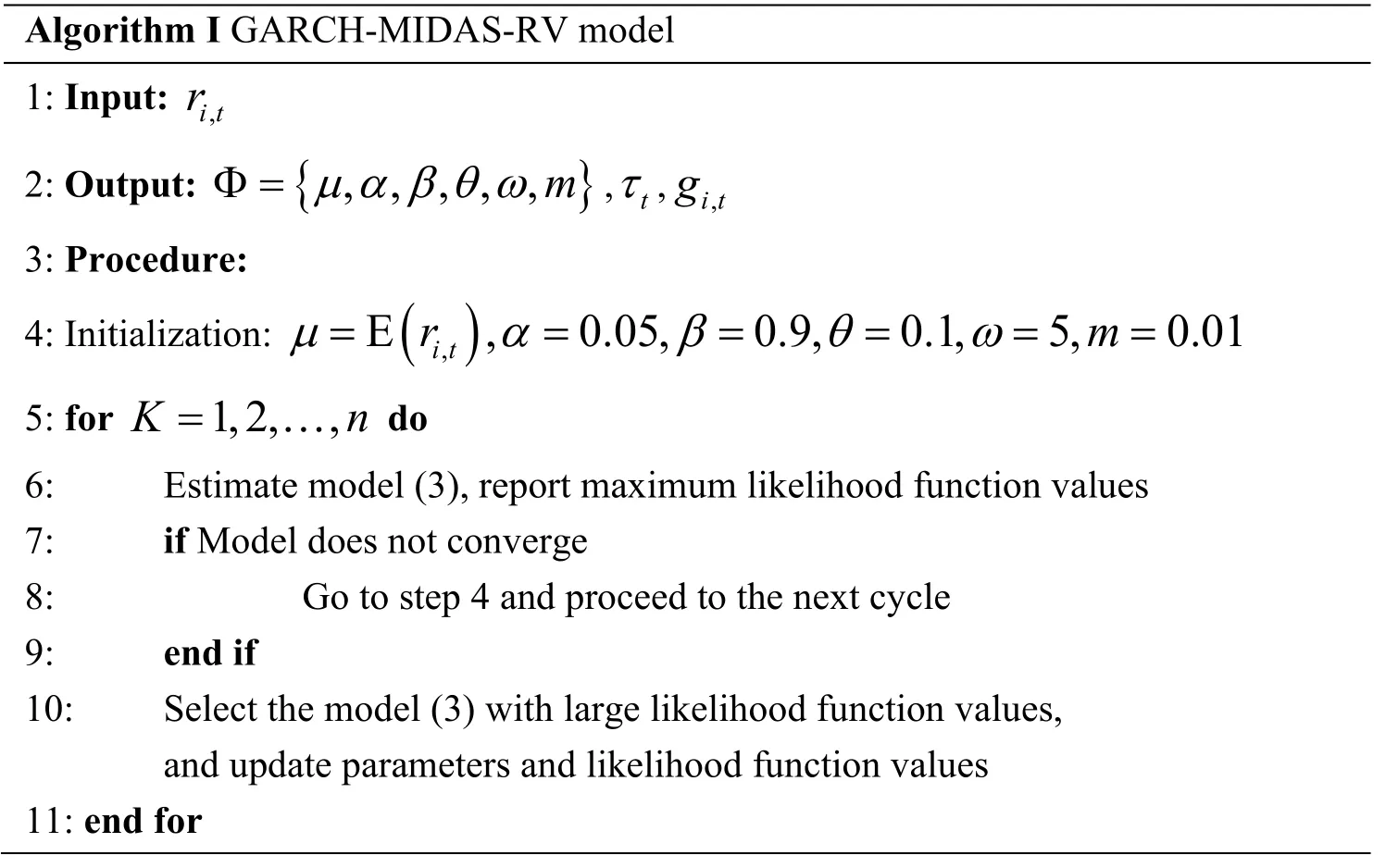
Algorithm I GARCH-MIDAS-RV model 1:Input:,i tr 2:Output:{ },,,,,mµ α β θ ω Φ=,tτ,,i tg 3:Procedure:4:Initialization:(),E,0.05,0.9,0.1,5,0.01 i tr m µ α β θ ω======5:for 1,2,,K n=… do 6:Estimate model (3),report maximum likelihood function values 7:if Model does not converge 8:Go to step 4 and proceed to the next cycle 9:end if 10:Select the model (3) with large likelihood function values,and update parameters and likelihood function values 11:end for

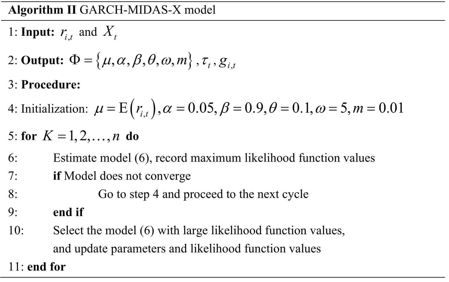
Algorithm II GARCH-MIDAS-X model 1:Input:,i tr and tX 2:Output:{ },,,,,mµ α β θ ω Φ=,tτ,,i tg 3:Procedure:4:Initialization:(),E,0.05,0.9,0.1,5,0.01 i tr m µ α β θ ω======5:for 1,2,,K n=… do 6:Estimate model (6),record maximum likelihood function values 7:if Model does not converge 8:Go to step 4 and proceed to the next cycle 9:end if 10:Select the model (6) with large likelihood function values,and update parameters and likelihood function values 11:end for

4 Experiment

4.1 Data

The high-yield bond data used in the experiments were gathered from the S＆P U.S.High Yield Bond Index4HYBX data comes from Gormus A,Nazlioglu S,Soytas U.High-Yield Bond and Energy Markets.Energy Economics,2018,69:101-110.(denoted as HYBX) over the period from May 17,2005 to June 22,2015.For U.S.economic policy uncertainty index and classification uncertainty index,we considered monetary policy,taxes,government spending and financial regulation5Economic policy uncertainty index and classification uncertainty index are from http://www.policyuncertainty.com,and the dataset was collected from May 2005 to June 2015,totally 122 monthly observations.The log return of HYBX price is defined by ri,t=log (Pi,t/Pi-1,t),where Pi,tand Pi-1,trepresent the price of the HYBX on the i th and 1i- th day of the t th month.

As shown in Tab.1.and Fig.1,the ADF test shows the return and realized volatility of high-yield bonds are stationary,while economic policy uncertainty,taxes and financial regulation are non-stationary.

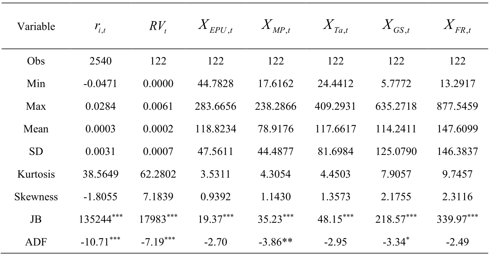
Table 1:Summary statistics of variables

XEPU,t,XMP,t,XTa,t,XGS,tand XFR,tindicate economic policy uncertainty,monetary policy,taxes,government spending and financial regulation,respectively.RVtrepresents the realized volatility of the ri,t.

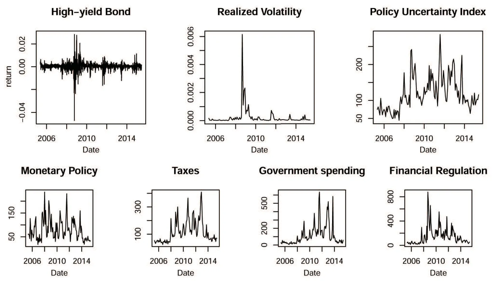
Figure 1:Time series of all variables

4.2 Models estimation

We selected a fixed time span including 22 trading days per month.In the GARCH (1,1) model,the short-term component used11ω=and an estimated value of2ω .The lag order was obtained according to the likelihood function value.For a monthly explanatory variable,12K=means that the lag order of explanatory variable in the MIDAS is 12 months.Moreover,we used root mean square error (RMSE) to measure the prediction effect,defined by,where T is a sample size,and σt2are the estimated and realized values of the volatility,respectively.Tab.2 reports the estimated results of the GARCH-MIDAS model based on the realized volatility of highyield bonds,economic policy uncertainty and other four macroeconomic variables.

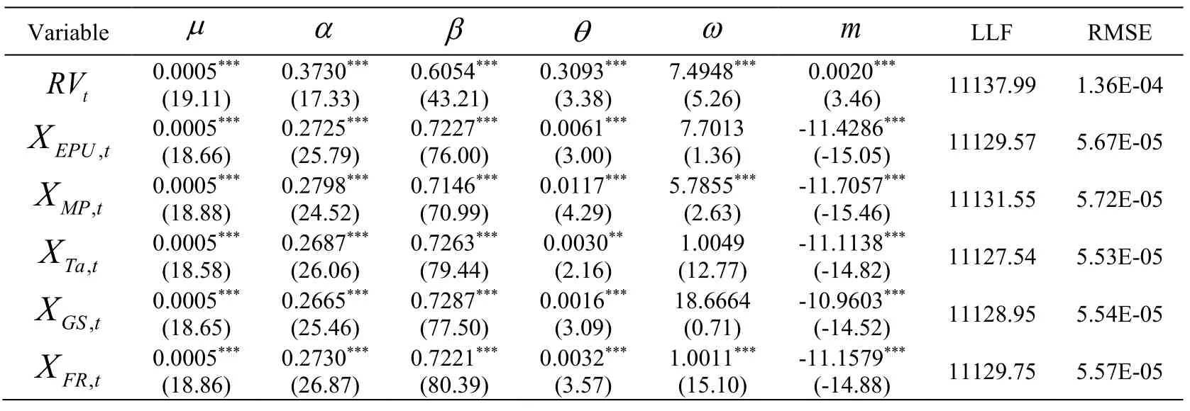
Table 2:Single factor mixed volatility model regression results

It can be seen from Tab.2 that the values of µ in the mixed volatility model with different explanatory variables are 0.5%,which implies that these models effectively capture the fluctuation of high-yield bonds.From the value of θ,it can be found that realized volatility of high-yield bonds,economic policy uncertainty and other four macroeconomic variables are positively correlated with the long-term components of the volatility of high-yield bonds.Moreover,these regression results show that the volatility of high-yield bonds is higher with the fluctuation of economic policy uncertainty,monetary policy,taxes,government spending and financial regulation,respectively.

Figure 2:Total volatility and long-term compositions of high-yield bond return fitted by mixed volatility models in full samples

In Fig.2,the dotted line indicates the total volatility of the high-yield bonds,and the solid line indicates the secular volatility denoted by long-term components volatility of high- yield bonds estimated by the mixed volatility model,i.e.,τt.It can be seen that the long- term component of the volatility has the same trend as the total volatility,which implies that the long-term component can reflect the overall trend of the total volatility.Particularly,economic policy uncertainty and monetary policy can fit better than other variables.

4.3 Robust

As can be seen from Fig.1,due to the impact of the global financial crisis in 2008,both the return and realized volatility of high-yield bonds and economic policy uncertainty index change more sharply.In order to test the robustness of the regression results,we divided the full sample period between May 2005 and June 2015 into two subsamples T1and T2with the cut-off point at September 2008,and constructed the models in the same way on the two subsamples.The results are listed in Tab.3 and Tab.4.

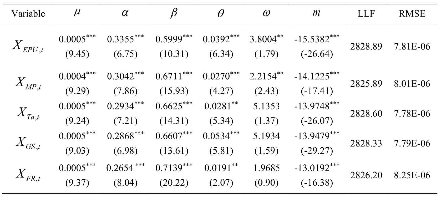
Table 3:Single factor mixed volatility model regression results in subsample 1T

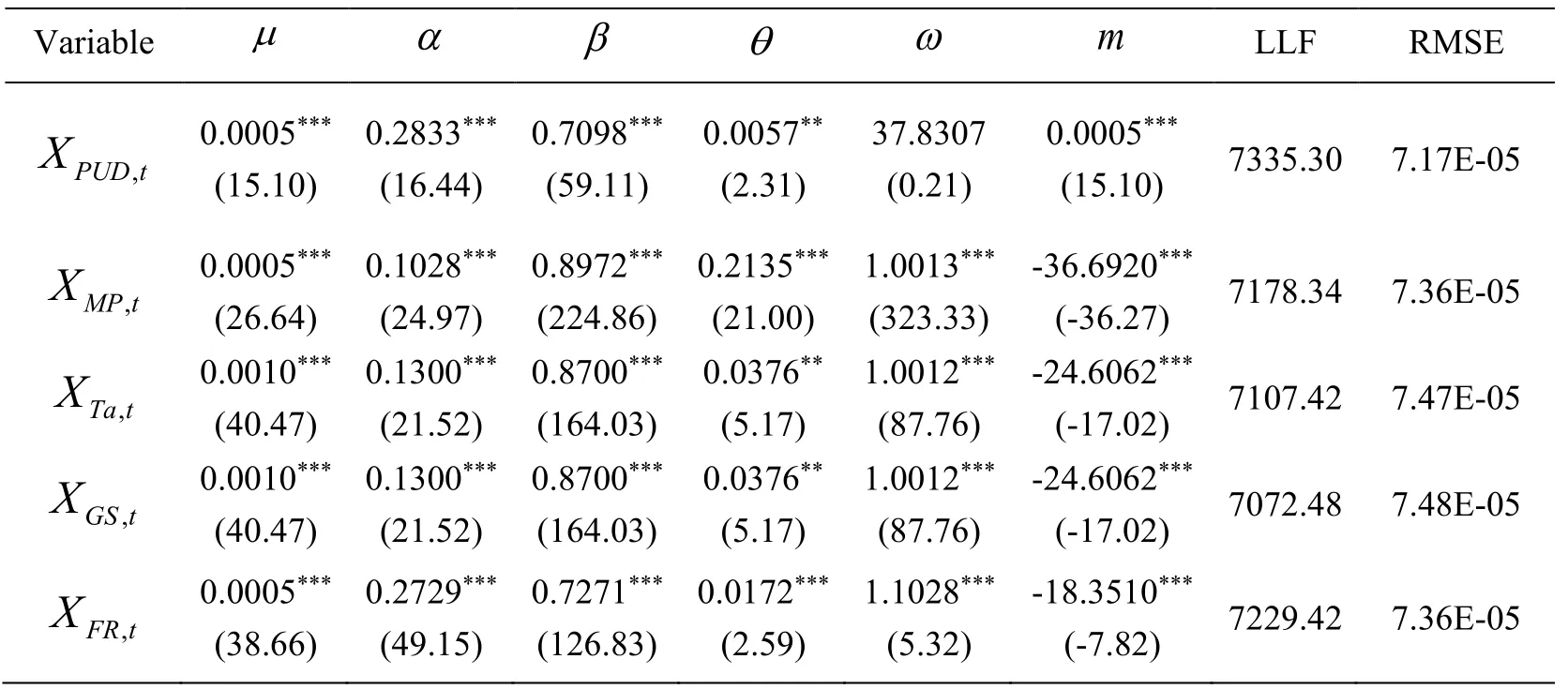
Table 4:Single factor mixed volatility model regression results in subsample 2T

Tab.3 and Tab.4 report regression results of the mixed volatility model in subsamples T1and T2with economic poli cy uncertainty,monetary policy,taxes,government spending and financial regulation.The results show that most of the parameters in the different subsamples are significant and correspond to the symbols of the regression parameters of the full sample in Tab.2,which implies that the regression results are robust.Especially,the value µ of taxes and government spending in subsample T2is larger,which implies that after financial crisis,the long-term components of taxes and government spending for the volatility of high-yield bonds is smaller.Moreover,the long-term effects of economic policy uncertainty,taxes,government spending and financial regulation on high-yield bonds are respectively consistent in the two subsamples,while the impact of monetary policy on high-yield bonds after financial crisis is stronger than that on highyield bonds before financial crisis.

In addition,the total volatility and long-term component volatility of high-yield bond return estimated by the mixed volatility model in the two subsamples are plotted,as shown in Fig.3.

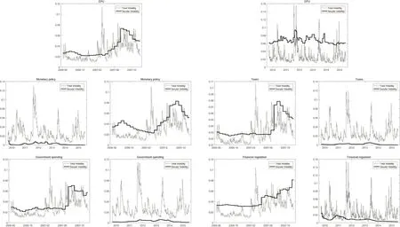
Figure 3:Total volatility and long-term components of high-yield bonds return fitted by mixed volatility models in two subsamples

In Fig.3,the dotted line and the solid line represent the total volatility and the secular volatility denoted by long-term component volatility of high-yield bonds fitted by the mixed volatility model,respectively.It can be found that for economic policy uncertainty index,monetary policy,taxes,government spending and financial regulation,the total volatility of high-yield bonds is almost consistent with the long-term component volatility in two different subsamples.

5 Conclusion

In order to avoid the information leakage caused by the same frequency data,we have used GARCH- MIDAS models with a decomposition of a volatility into short-term highfrequency components and long-term low-frequency components to examine the relationship between low-frequency macroeconomic variables and high-frequency financial market volatility.Moreover,based on two types of GARCH-MIDAS models,we have investigated the impact of economic policy uncertainty on the volatility of highyield bond market.The empirical results show that both the realized volatility of highyield bonds and the macroeconomic factors are positively correlated with the long-term components of high-yield bonds.This result indicates that investors can predict the volatility of high-yield bonds from the macroeconomic information.

Acknowledgement:This work was supported by National Natural Science Foundation of China (Nos.71461005,71561008),National Social Science Foundation of China (No.17BGL234) and Innovation Project of Guangxi Graduate Education (No.YCSW2017143).

References

Arouri,M.;Estay,C.;Rault,C.;Roubaud,D.(2016):Economic policy uncertainty and stock markets:long-run evidence from US.Finance Research Letters,vol.18,pp.136-141.

Baker,S.R.;Bloom,N.;Davis,S.J.(2016):Measuring economic policy uncertainty.Quarterly Journal of Economics,vol.131,no.4,pp.1593-1636.

Blumem,M.E.;Keim,D.B.;Patel,S.A.(1991):Returns and volatility of low-grade bonds 1977-1989.The Journal of Finance,vol.46,no.1,pp.49-74.

Colombo,V.(2013):Economic policy uncertainty in the US:does it matter for the euro area? Economics Letters,vol.121,no.1,pp.39-42.

Conrad,C.;Loch,K.;Rittler,D.(2014):On the macroeconomic determinants of long- term volatilities and correlations in U.S.stock and crude oil markets.Journal of Empirical Finance,vol.29,pp.26-40.

Dakhlaoui,I.;Aloui,C.(2016):The interactive relationship between the US economic policy uncertainty and BRIC stock markets.International Economics,vol.146,pp.141-157.

Ding,Z.;Granger,C.W.J.(1996):Modeling volatility persistence of speculative returns:a new approach.Journal of Econometrics,vol.73,no.1,pp.185-215.

Downing,C.;Underwood,S.;Xing,Y.(2009):The relative informational efficiency of stocks and bonds:an intraday analysis.Journal of Financial and Quantitative Analysis,vol.44,no.5,pp.1081-1102.

Engle,R.F.;Ghysels,E.;Sohn,B.(2013):Stock market volatility and macroeconomic fundamentals.Review of Economics and Statistics,vol.95,no.3,pp.776-797.

Engle,R.F.;Rangel,J.G.(2008):The spline-garch model for low-frequency volatility and its global macroeconomic causes.Review of Financial Studies,vol.21,no.3,pp.1187-1222.

Fridson,M.S.;Garman,M.C.(1998):Determinants of spreads on new high-yield bonds.Financial Analysts Journal,vol.54,no.2,pp.28-39.

Ghysels,E.;Santa-Clara,P.;Valkanov,R.(2006):Predicting volatility:getting the most out of return data sampled at different frequencies.Journal of Econometrics,vol.131,no.1,pp.59-96.

Ghysels,E.;Sinko,A.;Valkanov,R.(2007):Midas regressions:further results and new directions.Econometric Reviews,vol.26,no.1,pp.53-90.

Gormus,A.;Nazlioglu,S.;Soytas,U.(2018):High-yield bond and energy markets.Energy Economics,vol.69,pp.101-110.

Hong,Y.M.;Lin,H.;Wu,C.C.(2012):Are corporate bond market returns predictable? Journal of Banking and Finance,vol.36,no.8,pp.2216-2232.

Liu,W.J.;Xu,Y.;Yang,C.N.;Gao,P.P.;Yu,W.B.(2018):An efficient and secure arbitrary n-party quantum key agreement protocol using bell states.International Journal of Theoretical Physics,vol.57,no.1,pp.195-207.

Nieto,B.;Novales,A.;Rubio,G.(2015):Macroeconomic and financial determinants of the volatility of corporate bond returns.Quarterly Journal of Finance,vol.5,no.4,pp.1-41.

Tu,Y.;Lin,Y.;Wang,J.;Kim,J.(2018):Semi-supervised learning with generative adversarial networks on digital signal modulation classification.Computers,Materials ＆ Continua,vol.55,no.2,pp.243-254.

Wisniewski,T.P.;Lambe,B.J.(2015):Does economic policy uncertainty drive CDS spreads? International Review of Financial Analysis,vol.42,pp.447-458.

Zhang,T.;Wu,W.(2014):The asymmetric predictability of high-yield bonds.North American Journal of Economics and Finance,vol.29,pp.146-155.