Forecasting Damage Mechanics By Deep Learning

DuyenLeHienNguyen,DieuThiThanhDo,JaehongLee,TimonRabczukandHungNguyen-Xuan,

Abstract: We in this paper exploit time series algorithm based deep learning in forecasting damage mechanics problems.The methodologies that are able to work accurately for less computational and resolving attempts are a significant demand nowadays.Relied on learning an amount of information from given data,the long short-term memory (LSTM) method and multi-layer neural networks (MNN) method are applied to predict solutions.Numerical examples are implemented for predicting fracture growth rates of L-shape concrete specimen under load ratio,single-edge-notched beam forced by 4-point shear and hydraulic fracturing in permeable porous media problems such as storage-toughness fracture regime and fracture-height growth in Marcellus shale.The predicted results by deep learning algorithms are well-agreed with experimental data.

Keywords: Damage mechanics,time series forecasting,deep learning,long short-term memory,multi-layer neural networks,hydraulic fracturing.

1 Introduction

Damage mechanics has been considered as an important method for estimating the behaviour of materials and structures.The causes of most damages are human errors during design,construction or operation the structures,impact of nature,chemical action,use inappropriate materials and errors in stress analysis,etc.Damage induces the degradation of strength and stiffness that can be the cause of fracture of the structures [Lemaitre (1992);Valliappan,Murti and Wohua (1990)].The damage mechanics can represent initiation and propagation phases.This theory has been proposed to study the behaviour of brittle fracture,ductile fracture,creepy fracture and fatigue failure.Lemaitre [Lemaitre (1984)] defined a damage variable in continuum mechanics and derived an equation that performs the relevance of a damage variable altering ratio to cycle fatigue to effective stress.This method has been extended and applied for predicting fatigue thresholds of connected joints by Abdel Wahab et al.[Abdel Wahab,Ashcroft,Crocombe et al.(2001)].Johnson [Johnson (1992)] proposed the continuum damage mechanics based cell structure approach for investigation of fracture in plates.Tang et al.[Tang,Tham,Lee et al.(2002)] combined flow,stress and damage to analyse the fluid flow and damage evolution in rock subjected to hydraulic fracturing.

It can be said that in damage mechanics fracture growth and life failures are complicated to accurately measure.A number of numerical methods have been employed in damage evolution problems such as phase-field,extended finite element method (X-FEM),extended isogeometric analysis (X-IGA),meshfree method,particle method,singular edge-based smoothed finite element method (sES-FEM),scaled boundary finite element methods [Besson (2009);Jing (2003)].Nguyen-Thanh et al.[Nguyen-Thanh,Valizadeh,Nguyen et al.(2015)] provided X-IGA to cover the singular field appeared nearby the crack tip of thin shell structures.Nguyen-Xuan et al.[Nguyen-Xuan,Liu,Bordas et al.(2013)] proposed the adaptive singular ES-FEM to improve solutions that just use a number of nodes.Huynh et al.[Huynh,Tran,Zhuang et al.(2019)] investigated the use of X-FEM combined polygonal mesh to simulate large strain damage for hyper-elastic materials.The other approaches have been studied [Ambati,Gerasimov and De Lorenzis (2014);Natarajan,Wang,Song et al.(2015);Rao and Rahman (2000)].Each one has its own limitation,and generally,the primary drawback of them is rather expensive in computation that requires thousands of resolving attempts.The success of numerical models for damage mechanics mostly depends on aspects of fracture geometry,physical features of the individual fracture paths and fractured interfaces.Nowadays,numerical methods can address equation systems that are complicated and large-scale,but the physical quantitative representation of fractures in solid and hydraulic fracturing is still unsatisfactory [Jing(2003)].

For significantly reducing the cost of computation while conserving the accuracy,we propose time series forecasting based machine learning to predict damage behaviour in structures.In artificial intelligence area,machine learning is one of its subfields,which has been developing rapidly for recent five years.The definition of machine learning by Mitchell [Mitchell (1997)] is simply a computer program to learn to do a class of tasks via experience,respecting to performance measure if utilising its performance at tasks to measure program improving with experience.In other words,machine learning is strongly related to mathematical statistics models that use given sample data to efficiently solve a specific task without employing explicit methods.Most machine learning algorithms have many settings called hyper-parameters to control the behaviour of that algorithm.Based on data type to classify machine learning algorithms,mainly,three kinds are as follows:supervised learning,unsupervised learning and reinforcement learning.The space of applications artificial neural networks (ANN) and machine learning are in several sectors of computer vision,self-driving car,natural language processing,medical diagnosis,video game playing and so on.In 1989,the application of handwritten digits recognition successfully employed convolutional neural networks and backpropagation by LeCun et al.[LeCun,Boser,Denker et al.(1989)].From that,the US Postal Service automatically read the zip codes on mail envelopes in the 1990s.Bohn et al.[Bohn,Garcke,Iza-Teran et al.(2013)] analysed car smash simulation database by non-linear machine learning approaches that used principal manifold learning to reduce dimensions.This method is effective to nonlinear structure than principal component analysis because the full simulation execution in FEM has over one-million-node and hundreds of time steps that generate pretty high dimension.Voyant et al.[Voyant,Notton,Kalogirou et al.(2017)] reviewed support vector regression method,nearest neighbour neural network,decision tree learning,boosting,and random forests to forecast solar radiation.For predicting fracture growth,Younis et al.[Younis,Kamal,Sheikh et al.(2018)] used radial basic function neural network,Wang et al.[Wang,Zhang,Sun et al.(2017)] used extreme learning machine and genetic algorithms backpropagation networks,Mohanty et al.[Mohanty,Verma,Parhi et al.(2009)] forecasted fatigue lifetime of 2024 T3 and 7020 T7 aluminum alloys by ANN.Schwarzer et al.[Schwarzer,Rogan,Ruan et al.(2019)] used recurrent convolutional neural networks to predict fracture growth in brittle material.There are numerous applications of time series forecasting in computational mechanics.Jia et al.[Jia,Xu and Wang (2010)] studied the track geometry status forecast for developing track maintenance and repair plan.Kulkarni et al.[Kulkarni,Dhoble and Padole (2018)] applied this method into the wind speed forecast and turbine blade fatigue analysis.

In this study,we use deep learning approach to model behaviour of damage evolution.This approach is one of subfields of machine learning supported by ANN that has ability to train on and learn from data.The models of deep learning are long series of linear or non-linear functions applied sequentially.These operations are arranged into blocks called layers.The feature of layers are weights which learned and updated during the training process.We can refer the deep learning overview in Schmidhuber [Schmidhuber (2015)].Sirignano and Spiliopoulos [Sirignano and Spiliopoulos (2018)] merged deep learning into Galerkin method to solve partial differential equations.Anitescu et al.[Anitescu,Atroshchenko,Alajlan et al.(2019)] presented the use of ANN and adaptive collocation method for solving second order boundary value problems.Many applications have been provided in [Lenz,Lee and Saxena (2015);Ling,Kurzawski and Templeton (2016);Shen,Wu and Suk (2017)].We apply supervised learning algorithms in this study.A supervised learning is an algorithm learn to associate input values with output values,training data set contains both observed input and label or target output.

Observing examples of vectorand associated value or vector,algorithm learns how to predictfromby estimating a probability distribution.Through iterative optimization of a loss function,supervised learning algorithm finds out a function depended on parameters that would be employed to predict the output related to new input values.To correctly calculate the output values for inputs that are not included in the training dataset,an optimal function will be taken into account of the algorithm.Therefore,an algorithm that boosts the precision of its outputs or forecast over time is said to already have learned to perform that task.Two advanced methods,multi-layer neural networks and long short-term memory,will be applied to predict damage evolution in solid and hydraulic fracturing in porous media.

We divide this paper into five sections.The first one here is Section 1 for introduction.The damage models in mechanics are described in Section 2.They are the constitutive model for concrete,cohesive zone model,hydraulic fracturing in porous media and fracture-mapping technologies.Section 3 introduces the deep learning methods based multi-layer neural networks and long short-term memory.We implement,in Section 4,four numerical simulations of damage evolution problems by deep learning models which have been proposed as above,then compare the predicted results with experimental dataset in the references.There are some conclusions and future work in Section 5.

2 Damage models

2.1 Concrete constitutive model

Concrete is a composite material has a nonlinear inelastic property under multi-axial stress states.This is a favourite material in construction and is usually reinforced with other strong tension materials because it has the quite high compression,but weak tension.At low stress levels,the elasticity feature of concrete is intact,but gradual reducing as stress decreases.Based on plasticity theory forced by biaxial stress states to establish the constitutive model of concrete.It is extended by coupling tensile and compressive failure for unloading and reloading damage model.

We study a solid mechanics problem in domainsplit into two parts by an arbitrary discontinuity cutting [Nguyen-Xuan,Liu,Bordas et al.(2013)].The governing equations in the reference configuration can be defined by

2.2 Cohesive zone model

The schemes of the cohesive zone can represent the mixed mode crack behaviour.Two new surfaces are created in fracture process and singular stress appears at crack tip.The stress singularity can be removed by applying cohesive failure models,which have been originally introduced by Dugdale [Dugdale (1960)] and Barenblatt [Barenblatt (1962)].The cohesive zone model is presented in concrete and cement [Elices,Guinea,Gómez et al.(2002)] and applied to other materials such as polymers,metals,geomaterials [Hillerborg,Modéer and Petersson (1976)].The intrinsic method or initially elastic cohesive law and extrinsic method or rigid one are two fundamental methods to carry out cohesive crack models [Kubair and Geubelle (2003);Xu and Needleman (1993)].

The first approach consists of a traction-separation curve beginning at the original point with a hardening part,which shows the cohesive surface's rising opposition to be discontinuous.The cohesive traction is up to the greatest range with respect to a point where the material is failed at as the discontinuity is adequately obtained.After that,the traction-separation curve acts in accordance with a decreasing part which is related to the failure progress.We suppose that the cohesive traction is eliminated when the separation is at a critical condition.The region below the exponential curve is in respect of a fracture energy.The implementation of intrinsic cohesive law in FEM is simple due to the fixed geometry in the simulation process.However,this approach has some disadvantages.The predetermination of crack location is expected when applying this method.Thus,delamination problems are clear to predict,but dynamic fragmentations are impossible.The intrinsic cohesive laws need nonzero opening displacements to produce nonzero tractions;therefore,they are changing the material stiffness.

The extrinsic approach has been proposed to overwhelm the restrictions of the intrinsic one.This method only bases on the decreasing section of the cohesive law.Respestively,the cohesive traction is given by a material's failure strength.In this case,the unloading-reloading phase is also elastic and the region below the curve respects to a fracture energy as well.This approach model requires the alternative of its geometry in the simulation process,so many crack growths can be reproduced in arbitrary direction.The complicated implementation of rigid cohesive law is a significant drawback of this method.

2.3 Hydraulic fracture

The equation of the momentum in porous media domainis given as follows

The conservation fluid mass equation is defined by

Deriving the lubrication equation by inserting Eq.(5) without gravity into Eq.(4)

According to Tenzaghi [Terzaghi (1943)],the effective stress tensor is determined by

By applying poromechanics [Coussy (2004);Schrefler (2002)] to study the behaviour of surrounding fluid-saturated porous media,we obtain the hydro-mechanical equations as follows

2.4 Fracture mapping

The technologies of microseismic and microdeformation are used to constraint hydraulic fracture.Each method exploits difference information of the underground processes,but then they are used to verify and complementary for fracture-height growth data.

The use of microseismic is for post-fracture progress evaluation.Microseismic events are defined as very weak magnitude earthquakes recorded in very small areas.The microseismic mechanism is based on the alteration of location of reservoir when fracture movements occur [Warpinski (2009)].These movements are induced by changes to pressure and stress-strain conditions due to injecting fluid into or extracting fluid from wellbore.There are a number of sensors located along depth wells where the shale is fractured nearby.The two factors are compressional wave and shear wave which detected by sensors are attributes of miscroseisms.By using migration methods and grid search,the entry times and polarizations of wave are analysed to find out where the microseismic events initiated.The accurate velocity model is a principle part in measurement that can be provided by the monopole sonic log [Jones,Kendall,Bastow et al.(2014)].Besides,noise issues impact significantly to microseismic monitoring results,by small numbers of noise can decay fracture mapping.The geophones are set at depth to minimize the noise and enhance observed microseismic signal amplitudes.The downhole monitoring method requires close adequate wells to grant sufficiently the coverage of microseismic event location.

Microdeformation is the technology use sensitive tiltmeters to measure the very small displacement field on the ground and in the borehole as well cause by hydraulic fracture [Wright,Davis,Golich et al.(1998)].Tiltmeters have a variety of applications in construction and volcano monitoring.The principle of most of these instruments is using air bubble in a tube filled with liquid like a carpenter's level,but is embedded electronic sensors in to detect the tiniest changes in tilt.A number of tiltmeters are set up on the ground or observation wells to measure the rock surrounding deformation caused by hydraulic fracturing and to specify the fracture direction elements that are azimuth and dip.The tilt magnitudes combine with deformed zone width to determine the fracture depth and volume.In downhole tiltmeter,a few observation points are placed along the vertical well advance to the height of fracture than the deformation field [Sepehri,Agarwal and Davis (2015)].

The microseismic and microdeformation monitoring techniques,however,have some drawbacks.One is the operational expense is quite costly due to several source-receiver pairs requirement [Council (1996)].There is aboutof the hydraulic fracture stages on shales in US that were monitored by microseismic in comparison with other methods [Duncan and Eisner (2010);Yousefzadeh,Li and Aguilera (2015)].Another one is that the data which fracture parts involve in gas-flow to the well is not provided,just fracture dimensions [Ghaderi and Clarkson (2016)].

3 Deep learning

Deep learning is among the finest common methods of machine learning.Deep learning algorithms are mostly based on optimization funtions like stochastic gradient descent,Adam,Adagrad,RMSprop and Adadelta [Goodfellow,Bengio and Courville (2016)].Moreover,the loss function,neural network model and dataset are essential components to construct deep learning algorithms.

3.1 Multi-layer neural network (MNN)

Deep learning is specifically powered by neural networks.Actually,the neural network has a long history since the 1870s was originally proposed by Alexander Bain and William James.In the late 1950s,an American psychologist - Frank Rosenblatt,tried to develop a kind of machine which can possess human being characteristics in senses and remembering ability,and that machine is called “perceptron”.Single-layer perceptron combined with a step function is fine for simple linear problems,but it is not good at solving complicated ones such as non-linear outputs.Geoffrey Hinton et al.[Rumelhart,Hinton and Williams (1986)] introduced hidden layers in neural networks as neuron nodes between input and output layers.A hidden layer converts single-layer perceptron to multi-layer perceptron.An artificial neuron network in which its architecture includes one or more hidden layers is known as multi-layer neural network.Fig.1,for example,is a multi-layer neural network that has one input layer,two hidden layers and one output layer.

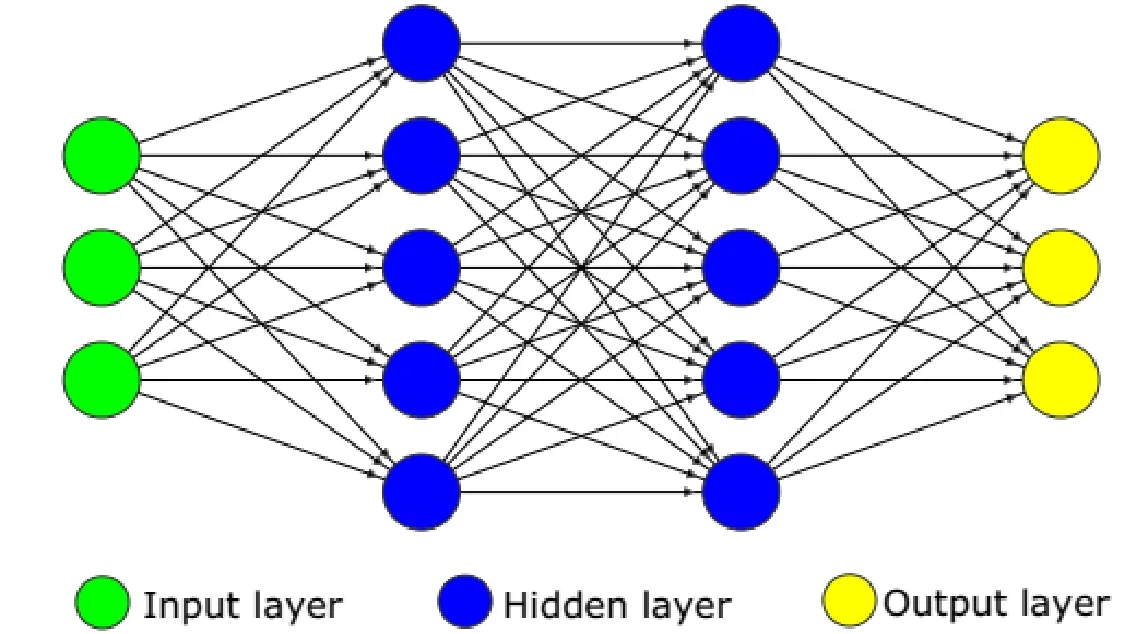
Figure 1:Multi-layer neural network architecture

To compute hidden layer values,we feedinto activation functionlike sigmoid,tanh,rectified linear unit (ReLU),softplus function.The activation functions have a great contribution in neural networks since they make the networks be non-linear,decide which nodes will be fired.Tab.1 shows some common activation functions.The value of hidden node th is by

Table 1:Activation functions

After hidden layers,we havevalues of hidden nodesand weight setand bias set,respectively.Having outputis as follows

Loss function (or cost function) is minimized during the training progress to evaluate how well the network performs on the training dataset and thus it can navigate itself correctly.The most common loss function used is mean square error betweenprediction valuesandtarget valuesby

There are other optimizers alter classical SGD such as adaptive gradient (Adagrad) [Duchi,Hazan and Singer (2011)],Adadelta [Zeiler (2012)],root mean square propagation (RMSprop) [Tieleman and Hinton (2012)],adaptive moment estimation (Adam) [Kingma and Ba (2014)].These ones have learning rate methods for each parameter,which provides a self-study approach,thus,significantly saves the cost in adjusting hyper-parameters manually.

3.2 Long short term memory (LSTM)

LSTM was firstly presented by Hochreiter and Schmidhuber [Hochreiter and Schmidhuber (1997)].LSTM uses gates in its architecture to control the memorizing procedure.The architecture of a LSTM unit is shown as in Fig.2,wheredenotes the last LSTM unit output,denotes memory from the last LSTM unit,is new current output andis new updated memory.Functionis used in core LSTM because it has the sustainable second derivative for a long span before vanishing.function can return the valueorwhich corresponds to forget or remember information.

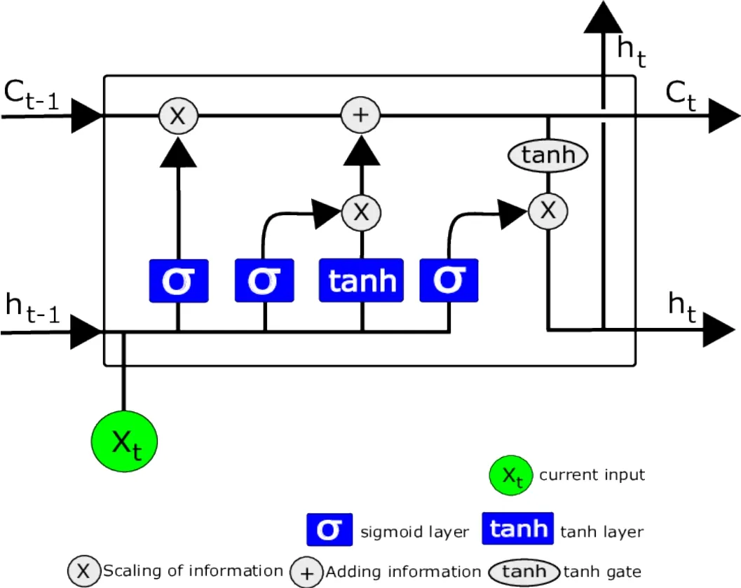
Figure 2:Architecture of a LSTM unit

Then,updating the old cell stateinto new updated memoryby multiplyingbyand adding the multiple offrom the first step into.The equation describes this process as below

The final stage is output result calculated through some steps.A sigmoid layer makes a decision which information of the cell state should be returned.In addition,a tanh function evaluates the cell state to generate possible values.After that,multiplying them by the output of the sigmoid layer.This process is illustrated by the following equations

4 Numerical examples

This section presents the productiveness of MNN and LSTM method through the four damage evolution problems in solid and hydraulic fracturing in porous media.All datasets in this study are taken from experiments and reliable measurement tools.A dataset is split up three parts:a training set,a test set and a validation set.The future values are predicted through learning from the training process.A test set is employed for evaluating efficiency of the model on a training dataset and make decision tuning the hyper-parameters.A validation set is to measure if the model is really good in reality.

4.1 Example 1:L-shape concrete specimen damage

This example is exploiting experimental data reported in Winkler et al.[Winkler,Hofstetter and Niederwanger (2001)] that describes the damage behaviour of the plain L-shape concrete sample.The inductive sensors are plug in four different points on the sample to measure displacements.The material properties are the Young's modulusGPa and Poisson's ratio.Let 50% of experimental dataset for training,the rest of fracture path will be predicted through two deep learning algorithms MNN and LSTM.Fig.3 depicts the predicted damage evolution and experimental data by MNN model uses 30 hidden nodes and optimization function Adam.The error for training is 2.406%,error for test is 1.279% and error for predicting compare to expected solutions is 3.222%.Forecast fracture path by LSTM algorithm uses the same configuration with MNN model,we obtain the training error is 2.333%,the test error is 1.165% and predicted error is 3.275%.As seen,there is no large difference in errors between these two algorithms.

Applying the model deep learning MNN and LSTM mentioned above to predicted the displacements as well.When we take 50% dataset for training,in which,10% for testing - 90% for training,note that the dataset contains 470 records,the validation errors by MNN method and LSTM are 8.007% and 2.875%,respectively.In this case,the LSTM works more precisely than MNN,although dataset passes through 100 epochs in LSTM,meanwhile,MNN model uses 1000 epochs.Convergence history and plotting difference between predicted values and expected ones by MNN are shown in Fig.4,by LSTM are indicated in Fig.5.The results are noted in Tab.2.

Figure 3:Predicting fracture growth of the L-shape concrete by MNN algorithm trained on 50% of the dataset

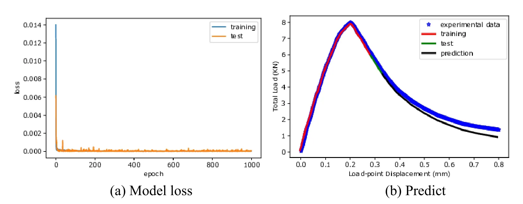
Figure 4:Convergence history and predictions of L-shape specimen displacement made by MNN trained on 50% of dataset compared to experimental data

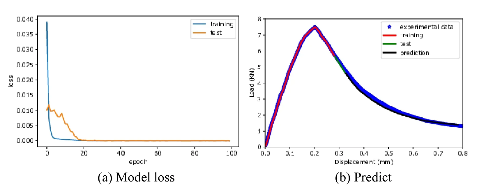
Figure 5:Convergence history and predictions of L-shape specimen displacement made by LSTM trained on 50% of dataset compared to experimental data

Table 2:The errors for predicting damage evolution and displacement of L-shape specimen using MNN and LSTM model training on 50% of the dataset

4.2 Example 2:fracture of a 4-point shear beam

The experimental results of 4-point shear beam (4PSB) fracture evolution were reported in Carpinteri et al.[Carpinteri,Valente,Ferrara et al.(1993);Naderi,Jung and Yang (2016)].The geometry,size (in),loading and boundary conditions of the test specimen is shown in Fig.6.The notch is created by a circular saw.This concrete beam has material properties Young's modulusMPa,Poisson ratioultimate tensile stressMPa and fracture energyN/m.

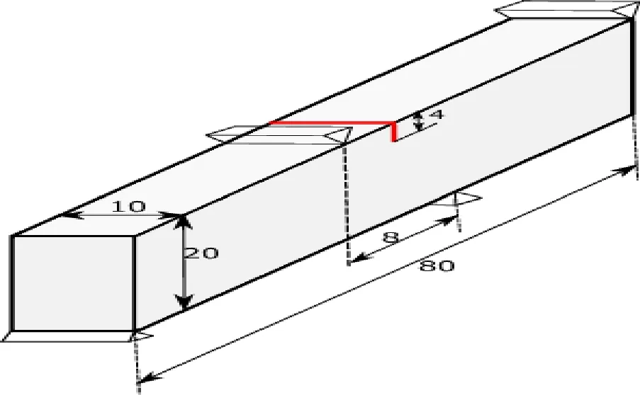
Figure 6:Single-edge-notched beam model forced by 4-point shear

In this example,the configuration of MNN and LSTM is one input layer-one hidden layer 60 units-one output layer,amount of epochs in MNN is 1000 and in LSTM is 100.To predict the damage propagation of 4PSB specimen,we let the machine learn on 70% of the actual dataset,therein 90% for training and 10% for testing,and optimize by Adam optimizer.Fig.7 plots the prediction from the training set,test set and validation set in comparison with the experimental database.Tab.3 shows the errors of predicting fracture growth of 4PSB by two deep learning algorithms.The validation errors are 0.363% for MNN and 1.370% for LSTM.

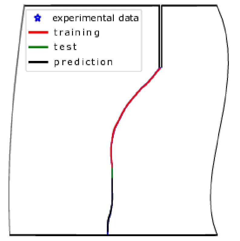
Figure 7:Predicting fracture evolution in example 4PSB using MNN model training on 70% of the dataset

Table 3:Compare errors for predicting fracture evolution in example 4PSB using MNN and LSTM model training on 70% of the dataset

The test continues to use these MNN and LSTM model to predict the displacement.Give training on 520 samples,test on 58 ones and validation on 250 ones.Minimizing loss function by different adaptive gradient algorithms Adam,Adagrad,Adadelta and RMSprop to evaluate which one is the most suitable for this example.The convergence history and the graphs of prediction with data from the experiment are depicted in Figs.8 and 9.The results are shown in the Tab.4.It can be seen easily that Adam optimizer works more effectively than Adagrad,Adadelta and RMSprop with prediction errors are 4.480% in LSTM and 12.489% in MNN.The use of MNN method returns the prediction errors are 18.168%,17.051%,18.169% in algorithms of Adagrad,Adadelta and RMSprop,respectively.By LSTM method,the prediction errors are 9.452% in Adagrad,13.493% in Adadelta and 10.156% in RMSprop.

Overall,the LSTM network using 70% dataset for training combined with Adam optimization function is the appropriate model for displacement forecast in 4PSB test example.

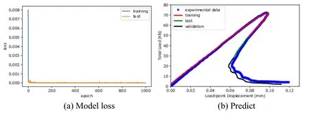
Figure 8:Convergence history and predictions of displacement made by MNN with Adam optimizer compared to the actual data

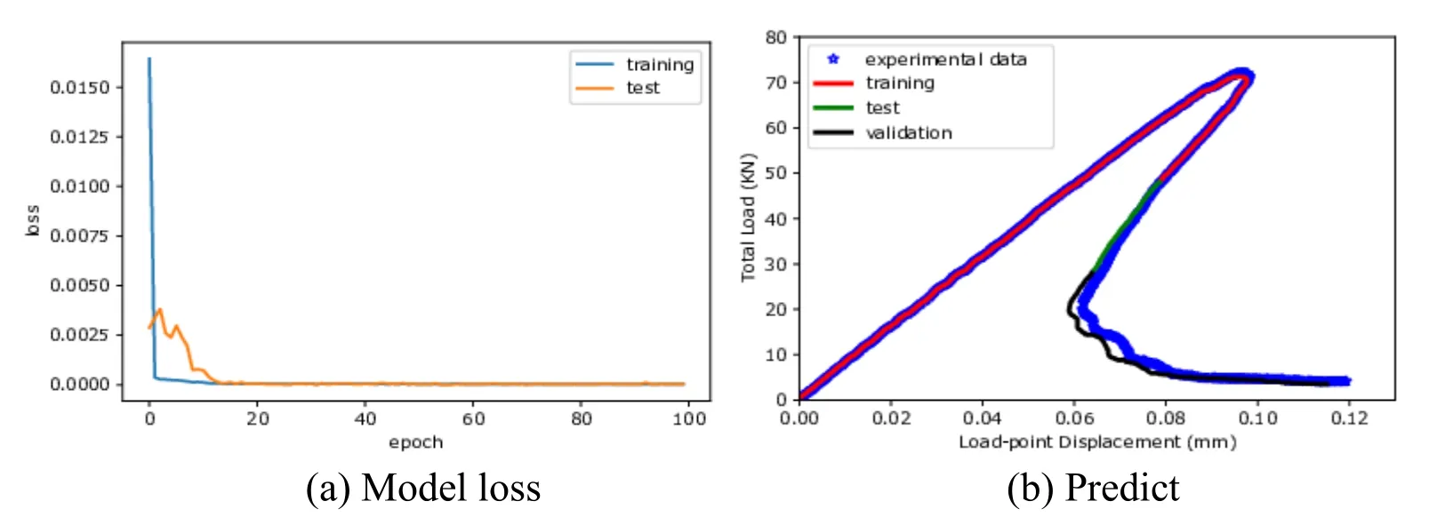
Figure 9:Convergence history and predictions of displacement made by LSTM with Adam optimizer compared to the actual data

Table 4:Comparing errors for predicting of displacement in example 4PSB using MNN and LSTM model training on 70% of the dataset with optimizers

4.3 Example 3:Storage-toughness dominated regime

There were studies the impact of specific permeability around porous media [Adachi and Detournay (2008);Bunger,Detournay and Garagash (2005);Garagash (2006)] before.This example predicts the fracture aperture and fracture length occur when an incompressible fluid is injected into a fracture base on analytical solutions introduced by Carrier and Granet [Carrier and Granet (2012)].We study the plain strain case and Kristianovich-Geertsma-de Klerk (KGD) fracture model displayed in Fig.10.In the figure,stands for fracture length,denotes the fracture aperture,is the fluid pressure in the fracture,far-field stressis perpendicular to the fracture andis injection rate assumed to be constant.The problem is symmetric toaxis,so we just compute a half of the space.The material properties are Young's modulusGPa,Poisson's ratio,Biot coefficient,Biot modulusMPa,injection rateGive a viscosityPa.s,permeabilityleak-off times,far-field stressMPa.We calculate the injection of 20 s to ensure the fracture path remains in the storage regime.

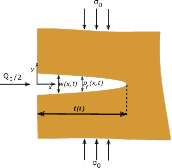
Figure 10:KGD hydraulic fracturing model

Let the training percentage is 30% of the dataset,therein the test part is 10%,we predict the fracture aperture in the rest of time interval by MNN and LSTM networks used 60 hidden nodes and Adam optimizer.For the convergence of errors and the output from training,test and validation tests by MNN model after 100 runnings (epochs) are shown in Fig.11,and for loop over 1000 epochs are depicted in Fig.13.Fig.12 and Fig.14 show the error convergences and prediction results from using LSTM model.The Tab.5 respectively shows that validation error for MNN model 100 epochs case is 2.481%,while 1000 ones return validation error is 3.460%;model LSTM 100 epochs and 1000 ones give the errors are 17.683% and 0.465%.Similarly,we increase the training percentage to be 50%.Fig.15 and Fig.17 illustrate history convergences and output predictions of MNN algorithm 100 epochs and 1000 ones,while the description of results from LSTM process 100 epochs is in Fig.16,and from 1000 runnings in LSTM is plotted in Fig.18.All the output errors are noted in Tab.6 where we see that the use of 1000 epochs is better than 100 ones in MNN model with mean square error 0.601% and 1.563%.The case of 1000 epochs in LSTM model outputs the greatest error value,2.745%.

When the epoch number increases,the more weight coefficients are altered in the neural network that can make the curve be under-fitting at first,then be optimal,and turn over-fitting one.This is the reason why the model of training on 30% of the dataset by MNN 1000 epochs is not as good as 100 epochs,and the result of 50% training on of dataset by LSTM 100 epochs is better than 1000 epochs.Overall,the ideal model for predicting fracture aperture in this example can be the LSTM model with training on 30%,loop dataset over 1000 epochs.

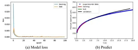
Figure 11:Convergence history and predictions of fracture aperture made by MNN with 30% dataset for training loop 100 epochs compared to experimental data

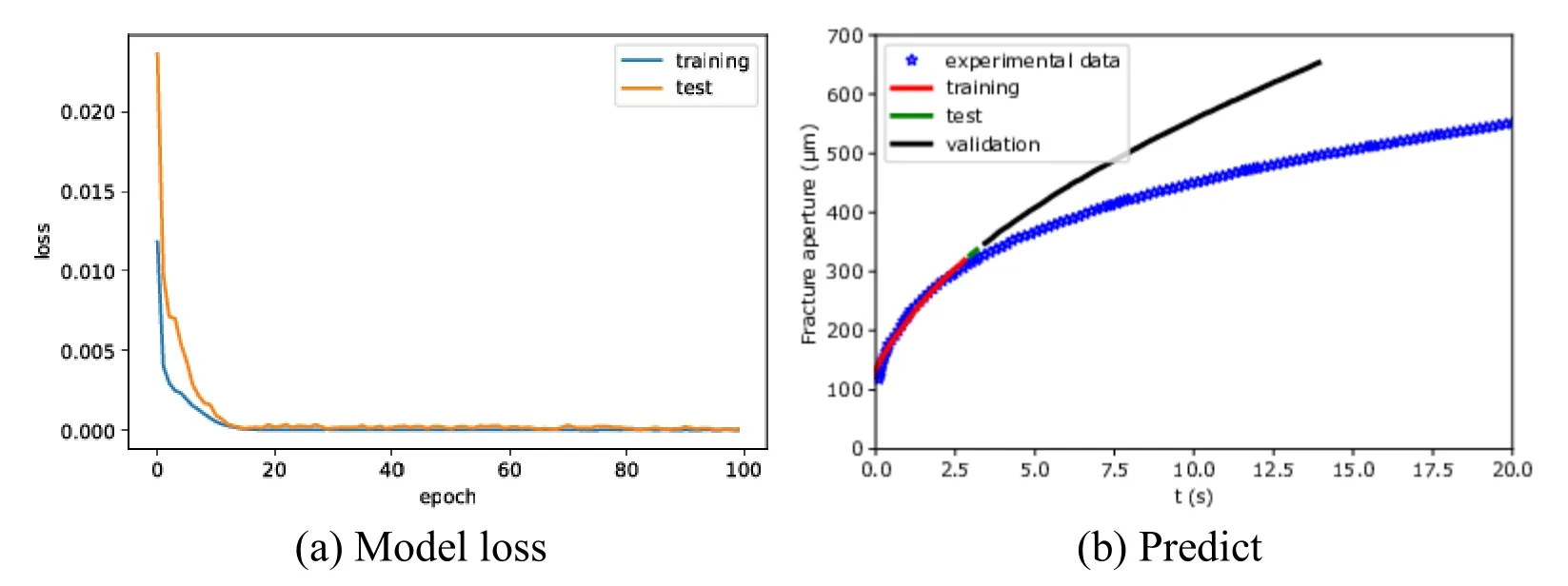
Figure 12:Convergence history and predictions of fracture aperture made by LSTM with 30% dataset for training loop 100 epochs compared to experimental data

Figure 13:Convergence history and predictions of fracture aperture made by MNN with 30% dataset for training loop 1000 epochs compared to experimental data

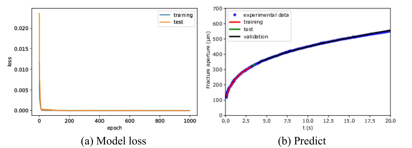
Figure 14:Convergence history and predictions of fracture aperture made by LSTM with 30% dataset for training loop 1000 epochs compared to experimental data

Table 5:The errors for predicting fracture aperture implemented by MNN and LSTM with training on 30% of the dataset,loop over 100 and 1000 epochs

Figure 15:Convergence history and predictions of fracture aperture made by MNN with 50% dataset for training loop 100 epochs compared to experimental data

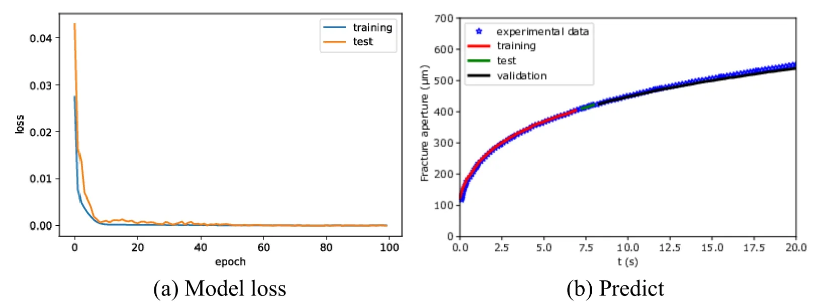
Figure 16:Convergence history and predictions of fracture aperture made by LSTM with 50% dataset for training loop 100 epochs compared to experimental data

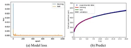
Figure 17:Convergence history and predictions of fracture aperture made by MNN with 50% dataset for training loop 1000 epochs compared to experimental data

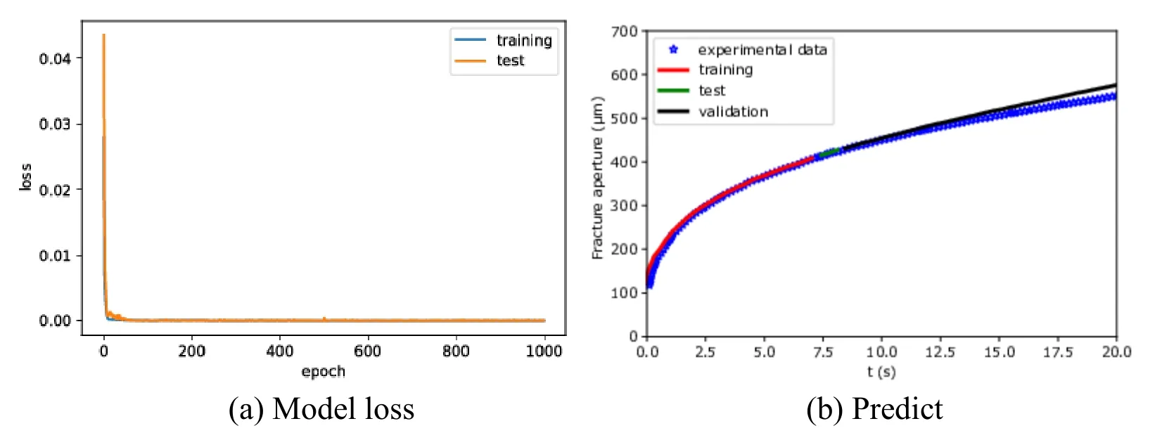
Figure 18:Convergence history and predictions of fracture aperture made by LSTM with 50% dataset for training loop 1000 epochs compared to experimental data

Table 6:The errors of predicting fracture aperture implemented by MNN and LSTM with training on 50% of the dataset,loop over 100 and 1000 epochs

It is done similarly to fracture length prediction.Firstly,30% of the input data is taken as training.The mean squared error convergence and output plots after 100 epochs in MNN model are shown in Fig.19,after 1000 epochs are in Fig.21.The graphs of Fig.20 and Fig.22 depict error convergences and prediction results by using LSTM model after 100 epochs and 1000 ones,respectively.The forecast errors by first training on 30% of the dataset are in Tab.7.Secondly,the set of training is on 50% of input data.For MNN method,the plots of history convergences and predictions from training,test and validation after 100 epochs and 1000 epochs are illustrated in Fig.23 and Fig.25,for LSTM method,are shown in Fig.24 and Fig.26.We can see all results in the Tab.8 that when loop over 100 runnings in MNN model returns validation error is 1.273% and 1000 epochs is 0.258%;in LSTM model,the validation errors are 1.875% for 100 epochs and 1.246% for 1000 ones.

The model of training on 50% of the input set by using MNN,60 hidden units and loop over 1000 epochs is the choice for predicting fracture length in this example.

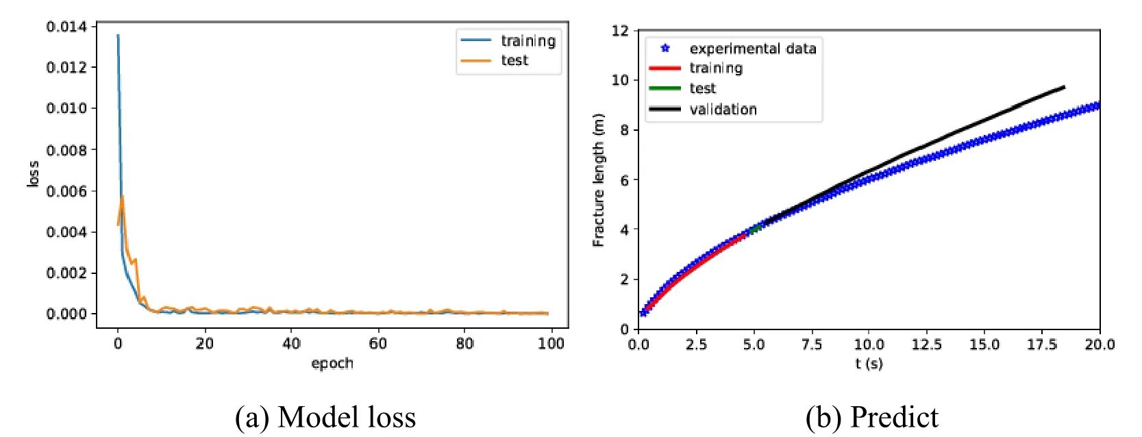
Figure 19:Convergence history and predictions of fracture length made by MNN with 30% dataset for training loop 100 epochs compared to experimental data

Figure 20:Convergence history and predictions of fracture length made by LSTM with 30% dataset for training loop 100 epochs compared to experimental data

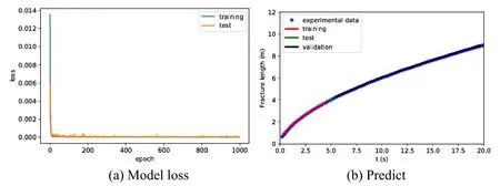
Figure 21:Convergence history and predictions of fracture length made by MNN with 30% dataset for training loop 1000 epochs compared to experimental data

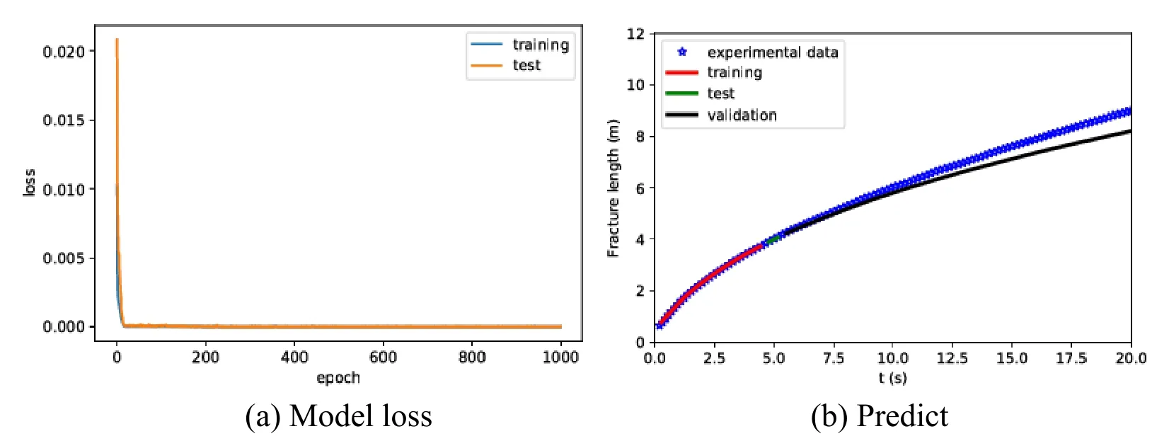
Figure 22:Convergence history and predictions of fracture length made by LSTM with 30% dataset for training loop 1000 epochs compared to experimental data

Table 7:The errors of predicting fracture length using MNN and LSTM training on 30% of the dataset,loop over 100 and 1000 epochs

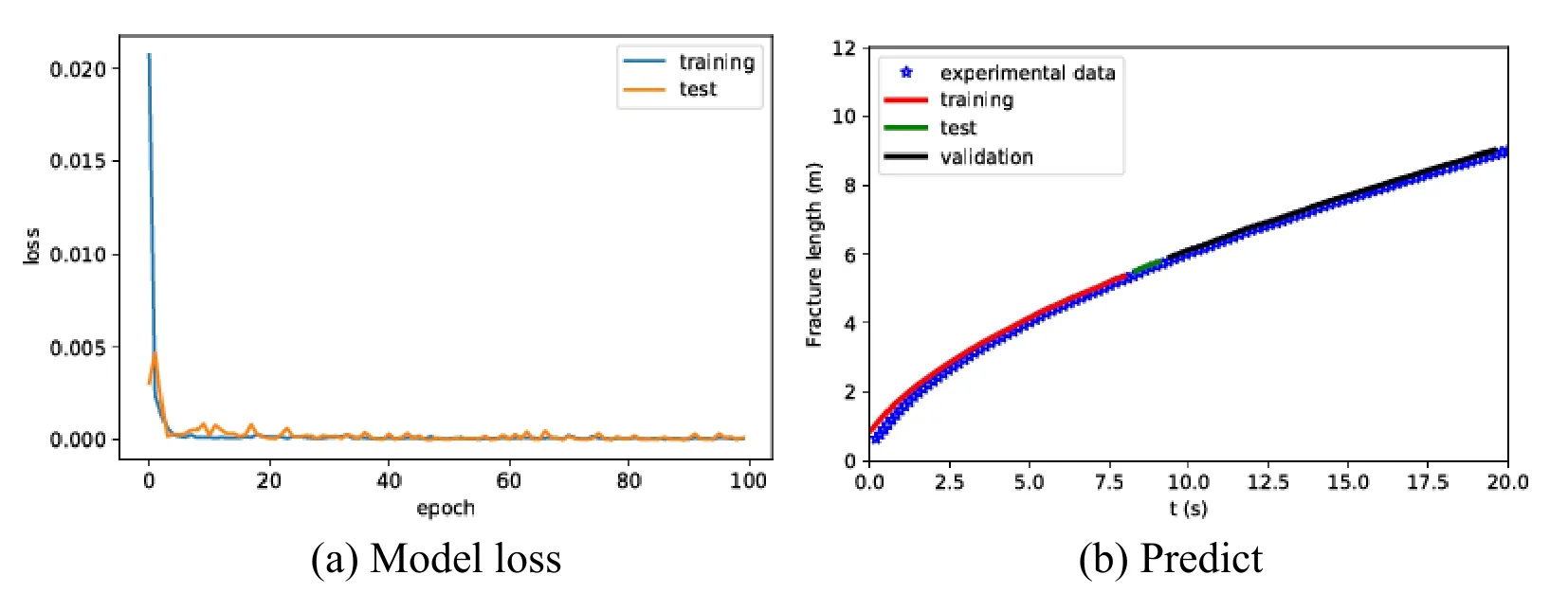
Figure 23:Convergence history and predictions of fracture length made by MNN with 50% dataset for training loop 100 epochs compared to experimental data

Figure 24:Convergence history and predictions of fracture length made by LSTM with 50% dataset for training loop 100 epochs compared to experimental data

Figure 25:Convergence history and predictions of fracture length made by MNN with 50% dataset for training loop 1000 epochs compared to experimental data

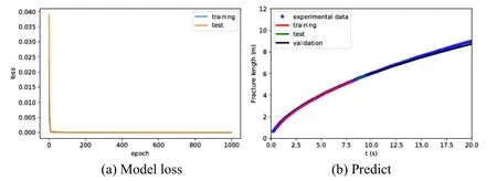
Figure 26:Convergence history and predictions of fracture length made by LSTM with 50% dataset for training loop 1000 epochs compared to experimental data

Table 8:The errors of predicting fracture length using MNN and LSTM training on 50% of the dataset,loop over 100 and 1000 epochs

4.4 Example 4:damage evolution of Marcellus shale

Fisher et al.[Fisher and Warpinski (2012)] indicated the real data of hydraulic fracture height evolution for Barnett,Woodford,Marcellus and Eagle Ford shale in North America.These values were collected in each reservoir in ten years from 2001 to 2010 by using microseismic and microdeformation fracture-mapping methods.Hydraulic fractures can get tall in hundreds of feet in vertical axis and lengthen in thousands of feet horizontally.

In this example,we consider the crack database of Marcellus shale in the Northeastern USA located in the depth from 5500 feet to around 8500 feet (1 foot0.3048 m) underground to predict the propagation of fracture tops and bottoms in hundreds of hydraulic fracturing stages.This shale layer has permeability in range 100-450 nanodarcy and very small pore size of tens nanometer.By reason of no permissive access to the main fracture-mapping data,the fracture height measurements in this study are obtained by digitising published figures.Using the model of MNN and LSTM network with 60 hidden neural nodes,Adam optimization function and dataset of first 150 fracture stages for training through 100 epochs to predict damage growth of next 200 stages cause by hydraulic fracture.In Fig.27,all depths are in true vertical depth,from 0 to 1000 ft is underground water layer,the shallowest fracture tops are approximately 4800 ft.Therefore,the fracturing of the Marcellus cannot impact to the aquifer.The errors of the forecast from the training set by MNN and LSTM model are 2.683% and 1.918%,test error is 1.413% for using MNN and 1.294% for LSTM.The fracture growth prediction in the rest of the stages gives the errors are 1.239% and 0.978% for algorithms MNN and LSTM,respectively.All results are recorded in Tab.9.

Figure 27:Predictions of hydraulic fracture propagation in Marcellus shale using LSTM model compared to fracture mapping data

Table 9:The errors of fracture growth predictions in Marcellus shale using MNN and LSTM model

5 Conclusions

Deep learning approach using time series forecasting to solve fracture propagation problems applied deep learning methods has been addressed.Two state-of-the-art MNN and LSTM model were investigated for predicting damage evolution in solid and hydraulic fracturing in porous media.The fracture growths in three-dimensional and hydraulic fracturing problems were precisely and rapidly predicted.The roles of optimization functions,epoch numbers and size of training data sets are important in the development of accurate prediction models.LSTM is more powerful,but also more expensive than MNN.Many problems in optimization neural network that should be studied are how to choose the right number of epochs for each type of dataset.The quality of the forecast would be improved by intergrating the solutions from different training methods with calibrated hyper-parameters.Moreover,a simulation results database of boundary and initial conditions patterns would be created to reproduce the most relevant cases of a particular problem.Afterward,machine learning algorithms would base on this database to automatically predict more general scenarios in future work.

Acknowledgment:The author would like to thank European Commission H2020-MSCA-RISE BESTOFRAC project for research funding.

References

Abdel Wahab,M.M.;Ashcroft,I.;Crocombe,A.D.;Shaw,S.J.(2001):Prediction of fatigue thresholds in adhesively bonded joints using damage mechanics and fracture mechanics.Journal of Adhesion Science and Technology,vol.15,no.7,pp.763-781.

Adachi,J.I.;Detournay,E.(2008):Plane strain propagation of a hydraulic fracture in a permeable rock.Engineering Fracture Mechanics,vol.75,no.16,pp.4666-4694.

Ambati,M.;Gerasimov,T.;De Lorenzis,L.(2014):A review on phase-field models of brittle fracture and a new fast hybrid formulation.Computational Mechanics,vol.55,no.2,pp.383-405.

Anitescu,C.;Atroshchenko,E.;Alajlan,N.;Rabczuk,T.(2019):Artificial neural network methods for the solution of second order boundary value problems.Computers,Materials ＆ Continua,vol.59,no.1,pp.345-359.

Barenblatt,G.I.(1962):The Mathematical theory of equilibrium cracks in brittle fracture.Advances in Applied Mechanics.Elsevier.

Besson,J.(2009):Continuum models of ductile fracture:a review.International Journal of Damage Mechanics,vol.19,no.1,pp.3-52.

Bohn,B.;Garcke,J.;Iza-Teran,R.;Paprotny,A.;Peherstorfer,B.et al.(2013):Analysis of car crash simulation data with nonlinear machine learning methods.Procedia Computer Science,vol.18,pp.621-630.

Bunger,A.;Detournay,E.;Garagash,D.(2005):Toughness-dominated hydraulic fracture with leak-off.International Journal of Fracture,vol.134,pp.175-190.

Carpinteri,A.;Valente,S.;Ferrara,G.;Melchiorrl,G.(1993):Is mode II fracture energy a real material property?Computers ＆ Structures,vol.48,no.3,pp.397-413.

Carrier,B.;Granet,S.(2012):Numerical modeling of hydraulic fracture problem in permeable medium using cohesive zone model.Engineering Fracture Mechanics,vol.79,pp.312-328.

Council,N.R.(1996):Rock fractures and fluid flow:contemporary understanding and applications.National Academies Press,Washington,D.C.

Coussy,O.(2004):Poromechanics.John Wiley ＆ Sons.

Duchi,J.C.;Hazan,E.;Singer,Y.(2011):Adaptive subgradient methods for online learning and stochastic optimization.Journal of Machine Learning Research,vol.12,pp.2121-2159.

Dugdale,D.S.(1960):Yielding of steel sheets containing slits.Journal of the Mechanics and Physics of Solids,vol.8,no.2,pp.100-104.

Duncan,P.M.;Eisner,L.(2010):Reservoir characterization using surface microseismic monitoring.GEOPHYSICS,vol.75,no.5,pp.75A139-175A146.

Elices,M.;Guinea,G.V.;Gómez,J.;Planas,J.(2002):The cohesive zone model:advantages,limitations and challenges.Engineering Fracture Mechanics,vol.69,no.2,pp.137-163.

Fisher,M.K.;Warpinski,N.R.(2012):Hydraulic fracture-height growth:real data.SPE Production ＆ Operations,vol.27,no.1,pp.8-19.

Garagash,D.I.(2006):Plane-strain propagation of a fluid-driven fracture during injection and shut-in:asymptotics of large toughness.Engineering Fracture Mechanics,vol.73,no.4,pp.456-481.

Ghaderi,S.M.;Clarkson,C.R.(2016):Estimation of fracture height growth in layered tight/shale gas reservoirs using flowback gas rates and compositions-Part I:model development.Journal of Natural Gas Science and Engineering,vol.36,pp.1018-1030.

Goodfellow,I.;Bengio,Y.;Courville,A.(2016):Deep Learning.MIT Press.

Hillerborg,A.;Modéer,M.;Petersson,P.E.(1976):Analysis of crack formation and crack growth in concrete by means of fracture mechanics and finite elements.Cement and Concrete Research,vol.6,no.6,pp.773-781.

Hochreiter,S.;Schmidhuber,J.(1997):Long Short-Term Memory.Neural Computation,vol.9,no.8,pp.1735-1780.

Huynh,H.D.;Tran,P.;Zhuang,X.;Nguyen-Xuan,H.(2019):An extended polygonal finite element method for large deformation fracture analysis.Engineering Fracture Mechanics,vol.209,pp.344-368.

Jia,C.;Xu,W.;Wang,H.(2010):Application of time series analysis in the analysis and forecasting of track geometry status.Applied Mechanics and Materials,vol.44-47,pp.3767-3770.

Jing,L.(2003):A review of techniques,advances and outstanding issues in numerical modelling for rock mechanics and rock engineering.International Journal of Rock Mechanics and Mining Sciences,vol.40,no.3,pp.283-353.

Johnson,E.(1992):Process region changes for rapidly propagating cracks.International Journal of Fracture,vol.55,no.1,pp.47-63.

Jones,G.A.;Kendall,J.M.;Bastow,I.D.;Raymer,D.G.(2014):Locating microseismic events using borehole data.Geophysical Prospecting,vol.62,pp.34-49.

Kingma,D.;Ba,J.(2014):Adam:a method for stochastic optimization.International Conference on Learning Representations.

Kubair,D.V.;Geubelle,P.H.(2003):Comparative analysis of extrinsic and intrinsic cohesive models of dynamic fracture.International Journal of Solids and Structures,vol.40,no.15,pp.3853-3868.

Kulkarni,P.;Dhoble,A.;M Padole,P.(2018):Deep neural network-based wind speed forecasting and fatigue analysis of a large composite wind turbine blade.Proceedings of the Institution of Mechanical Engineers,Part C:Journal of Mechanical Engineering Science,vol.233,no.8,pp.2794-2812.

LeCun,Y.;Boser,B.;Denker,J.S.;Henderson,D.;Howard,R.E.et al.(1989):Backpropagation applied to handwritten zip code recognition.Neural Computation,vol.1,no.4,pp.541-551.

Lemaitre,J.(1984):How to use damage mechanics.Nuclear Engineering and Design,vol.80,no.2,pp.233-245.

Lemaitre,J.(1992):A course on damage mechanics.Berlin:Springer-Verlag.

Lenz,I.;Lee,H.;Saxena,A.(2015):Deep learning for detecting robotic grasps.The International Journal of Robotics Research,vol.34,no.4-5,pp.705-724.

Ling,J.;Kurzawski,A.;Templeton,J.(2016):Reynolds averaged turbulence modelling using deep neural networks with embedded invariance.Journal of fluid mechanics,vol.807,pp.155-166.

Mitchell,T.M.(1997):Machine Learning.McGraw-Hill,New York.

Mohanty,J.R.;Verma,B.B.;Parhi,D.R.K.;Ray,P.(2009):Application of artificial neural network for predicting fatigue crack propagation life of aluminum alloys.Computational Materials Science and Surface Engineering,vol.1,no.3,pp.133-138.

Naderi,M.;Jung,J.;Yang,Q.(2016):A three dimensional augmented finite element for modeling arbitrary cracking in solids.International Journal of Fracture,vol.197,no.2.

Natarajan,S.;Wang,J.;Song,C.;Birk,C.(2015):Isogeometric analysis enhanced by the scaled boundary finite element method.Computer Methods in Applied Mechanics and Engineering,vol.283,pp.733-762.

Nguyen-Thanh,N.;Valizadeh,N.;Nguyen,M.N.;Nguyen-Xuan,H.;Zhuang,X.et al.(2015):An extended isogeometric thin shell analysis based on Kirchhoff-Love theory.Computer Methods in Applied Mechanics and Engineering,vol.284,pp.265-291.

Nguyen-Xuan,H.;Liu,G.R.;Bordas,S.;Natarajan,S.;Rabczuk,T.(2013):An adaptive singular ES-FEM for mechanics problems with singular field of arbitrary order.Computer Methods in Applied Mechanics and Engineering,vol.253,pp.252-273.

Rao,B.;Rahman,S.(2000):An efficient meshless method for fracture analysis of cracks.Computational Mechanics,vol.26,no.4,pp.398-408.

Rumelhart,D.E.;Hinton,G.E.;Williams,R.J.(1986):Learning representations by back-propagating errors.Nature,vol.323,no.6088,pp.533-536.

Schmidhuber,J.(2015):Deep learning in neural networks:an overview.Neural Networks,vol.61,pp.85-117.

Schrefler,B.(2002):Mechanics and thermodynamics of saturated/unsaturated porous materials and quantitative solutions.Applied Mechanics Reviews,vol.55.

Schwarzer,M.;Rogan,B.;Ruan,Y.;Song,Z.;Lee,D.Y.et al.(2019):Learning to fail:predicting fracture evolution in brittle material models using recurrent graph convolutional neural networks.Computational Materials Science,vol.162,pp.322-332.

Sepehri,J.;Agarwal,K.;Davis,E.(2015):The effect of reservoir layering on downhole microdeformation hydraulic fracture height measurements.SPE Annual Technical Conference and Exhibition.Society of Petroleum Engineers.

Shen,D.;Wu,G.;Suk,H.I.(2017):Deep learning in medical image analysis.Annual Review of Biomedical Engineering,vol.19,pp.221-248.

Sirignano,J.;Spiliopoulos,K.(2018):DGM:a deep learning algorithm for solving partial differential equations.Journal of Computational Physics,vol.375,pp.1339-1364.

Tang,C.A.;Tham,L.G.;Lee,P.K.K.;Yang,T.H.;Li,L.C.(2002):Coupled analysis of flow,stress and damage (FSD) in rock failure.International Journal of Rock Mechanics and Mining Sciences,vol.39,no.4,pp.477-489.

Terzaghi,K.(1943):Theoretical Soil Mechanics.John Wiley ＆ Sons.

Tieleman,T.;Hinton,G.(2012):Lecture 6.5-RMSprop:divide the gradient by a running average of its recent magnitude.Tech.Rep.

Valliappan,S.;Murti,V.;Wohua,Z.(1990):Finite element analysis of anisotropic damage mechanics problems.Engineering Fracture Mechanics,vol.35,no.6,pp.1061-1071.

Voyant,C.;Notton,G.;Kalogirou,S.;Nivet,M.L.;Paoli,C.et al.(2017):Machine learning methods for solar radiation forecasting:a review.Renewable Energy,vol.105,pp.569-582.

Wang,H.;Zhang,W.;Sun,F.;Zhang,W.(2017):A comparison study of machine learning based algorithms for fatigue crack growth calculation.Materials (Basel,Switzerland),vol.10,no.5.

Warpinski,N.(2009):Microseismic monitoring:inside and out.Journal of Petroleum Technology,vol.61,pp.80-85.

Winkler,B.;Hofstetter,G.;Niederwanger,G.(2001):Experimental verification of constitutive model for concrete cracking.Proceedings of The Institution of Mechanical Engineers Part L-journal of Materials-design and Applications,vol.215,no.2,pp.75-86.

Witherspoon,P.A.;Wang,J.S.Y.;Iwai,K.;Gale,J.E.(1980):Validity of cubic law for fluid flow in a deformable rock fracture.Water Resources Research,vol.16,no.6,pp.1016-1024.

Wright,C.A.;Davis,E.J.;Golich,G.M.;Ward,J.F.;Demetrius,S.L.et al.(1998):Downhole tiltmeter fracture mapping:finally measuring hydraulic fracture dimensions.SPE Western Regional Meeting.Society of Petroleum Engineers.

Xu,X.P.;Needleman,A.(1993):Void nucleation by inclusion debonding in a crystal matrix.Modelling and Simulation in Materials Science and Engineering,vol.1,no.2,pp.111-132.

Younis,H.B.;Kamal,K.;Sheikh,M.;Hamza,A.;Zafar,T.(2018):Prediction of fatigue crack growth rate in aircraft aluminum alloys using radial basis function neural network.2018 Tenth International Conference on Advanced Computational Intelligence,pp.825-830.

Yousefzadeh,A.;Li,Q.;Aguilera,R.(2015):Microseismic 101:monitoring and evaluating hydraulic fracturing to improve the efficiency of oil and gas recovery from unconventional reservoirs.SPE Latin American and Caribbean Petroleum Engineering Conference.Society of Petroleum Engineers.

Zeiler,M.D.(2012):ADADELTA:an adaptive learning rate method.arXiv preprint arXiv:1212.5701.