A Stochastic Numerical Analysis for Computer Virus Model with Vertical Transmission Over the Internet

Muhammad Shoaib Arif,Ali Raza,Wasfi Shatanawi ,Muhammad Rafiq and Mairaj Bibi

Abstract: We are presenting the numerical analysis for stochastic SLBR model of computer virus over the internet in this manuscript.We are going to present the results of stochastic and deterministic computer virus model.Outcomes of the threshold number C∗ hold in stochastic computer virus model.If C∗＜1 then in such a condition virus controlled in the computer population while C∗＞1 shows virus spread in the computer population.Unfortunately,stochastic numerical techniques fail to cope with large step sizes of time.The suggested structure of the stochastic non-standard finite difference scheme (SNSFD) maintains all diverse characteristics such as dynamical consistency,bounded-ness and positivity as well-defined by Mickens.On this basis,we can suggest a collection of plans for eradicating viruses spreading across the internet effectively.

Keywords: Computer virus model,stochastic modelling,stochastic techniques,stability.

1 Literature survey

A computer virus is a program that can copy itself and infect a computer without the permission or knowledge of the user.Virus stands for vital information resources under siege.A computer virus has two features as the potential to duplicate itself and the potential to affix itself to an alternative computer folder.They spread via disks,network or services such as email.Earlier viruses were propagated by computer programs or by hiding in floppy disks.Modern viruses transmit in a subtler way such as phishing which is a fraudulent practise of sending emails inquiring personal information [Patil and Jadhav 2014)].A virus-infected computer shows various symptoms.A small number of signs that may inform that a computer has the virus are slow response time,random hard drive crashes and great pop-up ads.A carefully engineered computer virus can disrupt production and cause billions of dollars in damages.For example,the con-flicker,also known as down up virus,which was discovered in 2008,had infected millions of computers across the world.The estimated damage was over $9.1 billion [Zhu,Yang and Ren (2012)].Viruses have evolved over a period.Their numbers are increasing each day,and they are becoming more sophisticated and harmful.Each new virus assimilates new features along with the old ones,thus making it more difficult to detect and erase [Albazzaz and Almuhanna (2016)].The computers that we usually use do not have adequate built-in security measures as compared to larger systems,thus leaving it to the users to purchase,install and utilise anti-virus software.Among significant types of computer viruses,the first type is called the boot sector virus.The boot sector is that first portion of our hard disk where routines to load our operating system reside.If these routines are disturbed or modified,our computer will not be able to work.As the name suggests,the boot sector virus modifies the boot sector program and is loaded in the memory whenever the computer is turned on.The virus is attached with the system executable files for example exe,.com etc.Chernobyl virus detects all the Microsoft office files and corrupts them.It also deletes the logical partition information of the disks.Users cannot access their files from the drives because of this virus.Logic bomb virus occurs only when a particular condition is met.The condition could be any date or any completion of the process (time).After the condition is met,the virus is invoked.This virus can be discovered by chance.Trojan horse virus is embedded in the computer programs.When we run these programs,this virus is activated.Its primary purpose is destruction.The Redlof virus is a polymorphic virus,which is written in VB Script (language).When instructions are being written,this virus is embedded in the programs.It corrupts the folder data file,which is the part of windows active desktop.An ideal structure of a computer virus holds three subroutines.The task of first sub-routine known as infect-executable,is to find executable files and infect them by copying its code into them.Next sub-routine,namely do-damage also called the virus payload,is a code which delivers the malicious part of the virus.The final sub-routine trigger-pulled inspects if the required conditions are met in order to deliver its payload [Patil and Jadhav (2014)].Much work has been done on the concept of computer viruses such as new techniques for virus detection and its prevention.New researches help us to understand how sophisticated viruses work.To inspect computer viruses,the compartment modelling technique of risky viruses was proposed by Cohen et al.[Cohen (1987);Murray (1988)].In last decade of the twentieth century,the authors were the first ones to typical the spreading behaviour of the computer virus.This paved the way for developing mathematical models for computer virus propagation [Billings,Spears and Schwartz (2002);Han and Tan (2010);Mishra and Jha (2007);Piqueira and Araujo (2009);Piqueira,Vasconcelos,Gabriel et al.(2008);Ren,Yang,Yang et al.(2012);Ren,Yang,Zhu et al.(2012);Wierman and Marchette (2004);Yuan and Chen (2008)].Just like any biological virus,the computer virus also contains a dormant period.During this period a single computer is vulnerable to a computer virus but is not infectious yet.An exposed computer,which is infected in dormancy,will not transmit the virus to other computers quickly;but it still can be infected.The delay used in some models of computer virus is also based on these characteristics.It shows that although the exposed computer does not infect other computers,it still has infectivity [Han and Tan (2010);Zhu,Yang and Ren (2012)].The authors proposed SLB and SLBS models in which they observed that the computer has latency,[Yang,Yang,Zhu et al.(2013);Yang,Yang,Wen et al.(2012)] and in this period of latency it also has infectivity.Multilayer networks can be responsible for spreading computer viruses.Examples of computer virus include mobile phone virus,which can use 3G,4G,Wi-Fi,or Bluetooth as a tool to communicate with other networks.Founded on the notion of the multilayer network,the IBMF (Individual-Based Mean Field) was applied to the SLBS model by Zhang [Zhang (2018)].A model was developed to expect the activities of worm on the network.A time-delayed SIQVD worm propagation model with variable infection rate was framed.This model can be utilized for internet worms [Yao,Fu,Yang et al.(2018)].Research has been conducted on the susceptible,latent,breaking-out,quarantine and susceptible (SLBQRS) computer virus model.Three finite-difference patterns have been used to solve the warm virus's system [Fatima,Ali,Ahmed et al.(2018)].HAM (Homotopy Analysis Method) has been utilized to solve the modified nonlinear SIR epidemiological model of computer viruses [Noeiaghdam,Suleman and Budak (2018)].The propagation mechanism of computer viruses is explored by the nodebased models.To examine the dynamic behaviour of a computer virus a model named SLIS which is node-based has also been proposed which demonstrated that the virus-free equilibrium is asymptotically or exponentially stable [Yu,Hu and Zeng (2019)].However,the influence of installing anti-virus software and the period of inactivity was not taken into account.The interaction frequency of afresh entered computers on the internet from vulnerable status to unprotected status is the same as that of vulnerable status entering into infected status.This tabloid works on the stochastic model of a computer virus,namely SLBRS model.It describes the vulnerability of uninfected computers and how they can get infected from the internet.We suppose that computers which join the internet are categorized into four classes.A threshold factor C∗is used to determine the dynamic characteristics of the suggested model.

Mathematical modelling has become very advanced to understand the viruses thoroughly.Formation of models and simulation allows us to analyze the sensitivity and make a comparison of conclusive opinions originating out of examples.Lots of studies are present on computer virus transmission dynamics models.Nonlinear initial value problems (IVPs) do not always,provide analytical solutions to specific issues and classical explicit finite-difference schemes such as Runge-Kutta,and Euler methods can bring confusion and unexpected fluctuations for discretization parameters [Mickens (1994,2005].Many types of research have been done on various computer virus models [Cai and Li (2010);Peng,He,Huang et al.(2013)].Stochastic differential equation models play an essential role in many branches of applied sciences such as industries,including population dynamics,finance,mechanics,medicine and biology as they provide an extra degree of realism compared to their deterministic counterpart [Bayram,Partal and Buyukoz (2018)].The usual quantitative explicit techniques for ODEs never maintain dynamical possessions as we have seen in the deterministic modelling.We have also seen that in explicit stochastic techniques do not maintain the dynamical possessions in the stochastic case.So,from this a question arises and need to research more:Could we develop the random emphatical scheme which maintains all the dynamical possessions? A rule introduced in the deterministic case,which has been used to start the notion stochastic nonstandard finite difference technique (SNSFD).These regulations were given by Mickens.This is the primary point of this paper.

This paper is divided into the following sections:

In Section 2,we have explained the deterministic computer model and its equilibria.Next section is about the formulation of the stochastic computer model.Section 4 explains the stochastic numerical techniques for stochastic computer virus model and their convergence analysis.Section 5 deals with the comparison of deterministic and stochastic numerical outcomes.Finally,in the last section,we shall present our deduction and give the future work.

2 Deterministic computer virus model

Here,we observe the deterministic computer virus model presented by Yang et al.[Yang,Zhang,Li et al.(2012)].Consider at any non-specific time t,the defined variables are S (exemplifies uninfected computers' fraction),L (exemplifies infected computers' fraction in latency),B (exemplifies infected computers' fraction which is broke-out) and R (exemplifies recovered computers' fraction with short-term immunity).The communication dynamics of computer virus model is illustrated below.

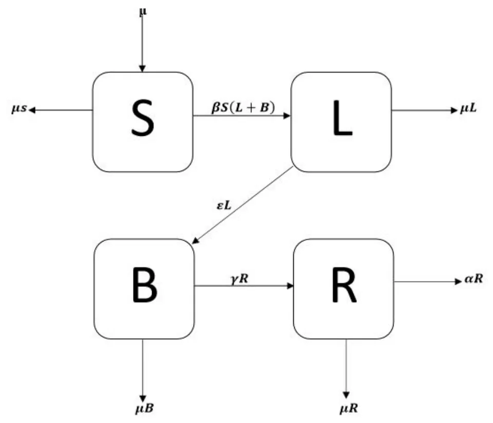
Figure 1:Flow map of computer virus model

The variables of the model are illustrated as µ (depicts the connected and withdrawn computer rate from the internet),β (pronounces the bilinear incidence rate of virus-free computers with infected computers),ε (pronounces the latent computers break out rate),r (pronounces the breaking out computers recovery rate) and α (pronounces the recovered computer rate that become virus-free).

The governing equations of the computer virus model as follows:

with conditions S ≥0,L ≥0,B ≥0,R ≥0

The reduced form of computer virus model is

with conditions S ≥0,L ≥0,B ≥0 and S+L+B ≤1.

2.1 Equilibria of the computer virus model

Given below are two ways of equilibrium points of computer virus model (3) as:

Virus-free equilibrium is V1=(S,L,B)=(1,0,,0)

Virus existence equilibrium is

C∗=C∗is the computer virus transmission generation number of model (3).It has an important part in virus dynamics.

3 Stochastic computer virus model

Let C(t)=[S,L,B]Tformulates the SDEs of computer virus model (3).We will determine the expectations Ε∗[∆C] and Ε∗[∆C∆CT].In order to find them the likely changes and their related transition probabilities are as follows (see Tab.1).

Table 1:Changes that may occur in the computer virus model

Following is the expectation of computer virus model (3):

The variance of the computer virus model is defined as Var= Ε∗[∆C∆CT]=

where

W11=μ(1-S)+βS(L+B)+α(1-S-L-B),W12=-βS(L+B),W13=0,W21=-βS(L+B),W22=βS(L+B)+(ε+μ)L,W23=-εL,.W31=0,W32=-εL,W33=εL+(γ+μ)B.

The SDE satisfy the diffusion processes,therefore,

Here,we have C(0)=Co=[0.2,0.7,0.1]T,0 ≤t ≤C as initial conditions and B as Brownian motion.

3.1 Euler maruyama technique

We used the parameters given by Yang et al.[Yang,Zhang,Li et al.(2012)] and euler maruyama technique presented in Maruyama [Maruyama (1955)],to analyze the numerical outcome of SDE (4).

The euler maruyama technique of (4) as:

where ∆t and ∆Bnis normally distributed between stochastic drift and stochastic diffusion,i.e.,∆Bn～N(0,1).The confidence interval holds the solution to stochastic differential equations for both equilibria as presented in the above numerical investigations.The outcome of deterministic computer virus model for the virus-free symmetry V1∗=(1,0,0) and C∗=0.0300 ＜1 may control the virus in the computer population through the internet.The viral equilibrium Ε1∗=(0.4353,0.5625,0.001607) and C∗=2.2974 ＞1 shows that the virus rapidly infects to the computer population through the internet.

4 Parametric perturbation of stochastic computer virus model

In this technique,we shall choose parameters from the system (3) and change into the random parameters with small noise as βdt=βdt+σdB.So,the stochastic system (3) is as follows [Allen,Allen,Arciniega et al.(2008)].

with initial conditions C(0)=[S(0),L(0),B(0)]T=[0.2,0.7,0.1]Twhere σ is casualness of each compartment of the computer virus model.

4.1 Equilibria of stochastic computer virus model

Two equilibria of the stochastic computer virus model (6) are as follows:

Virus-free equilibrium=(VFE)=(S,L,B)=(1,0,0).

Virus existence equilibrium= (VEE)=(So,Lo,Bo)

where,

4.2 Stochastic euler technique

The designed form of the model (6) as presented in Raza et al.[Raza,Arif and Rafiq (2019)]:

where “h” is represented as the discretized parameter of the method and i.e.,∆Bn～N(0,1).

4.3 Stochastic runge-kutta technique

The designed form of the model (6) as presented in Raza et al.[Raza,Arif and Rafiq (2019)]:

First Stage

Α1=h[μ(1-Sn)-βSn(Ln+Bn)+α(1-Sn-Ln-Bn)-σSn(Ln+Bn)∆Bn]

B1=h[βSn(Ln+Bn)-(ℰ+μ)Ln+σSn(Ln+Bn)∆Bn]

C1=h[ℰLn-(γ+μ)Bn]

Second Stage

Third Stage

Fourth Stage

Final Stage

where “h” is represented as the discretized parameter of the method and i.e.,∆Bn～N(0,1).

4.4 Stochastic NSFD technique

The recommended frameworks of SNSFD for the model (6) as presented in Raza et al.[Raza,Arif and Rafiq (2019)]:

where “h” is represented as the discretized parameter of the method and i.e.,∆Bn～N(0,1).

4.4.1Convergence analysis

Here we are to discuss the following theorems:

Theorem 1

For any given initial value (Sn(0),Ln(0),Bn(0)) ∈ R+3system (9) has a unique nonnegative solution (Sn,Ln,Bn) ∈ R+3on n ≥ 0,almost surely.

Theorem2

For all n ≥0 is a non-negative invariant set for the system (9).

Proof:Rewriting the system (9) as follows:

Adding the corresponding sides,we have

almost surely.

Theorem 3

The discrete dynamical system (9) has the same equilibria as that of the continuous dynamical system (6) for all n ≥0.

Proof:For solving the system (9),we get two states as follows:

VFE i.e.,V3=(Sn,Ln,Bn)=(1,0,0).

VPE i.e.,Ε3=(Sn,Ln,Bn).

where,

almost surely.

Theorem 4

The eigenvalues of the discrete dynamical system (9) lie in the unit circle for all n ≥0.

Proof:

We consider F,G,and H from the system (9) as follows:

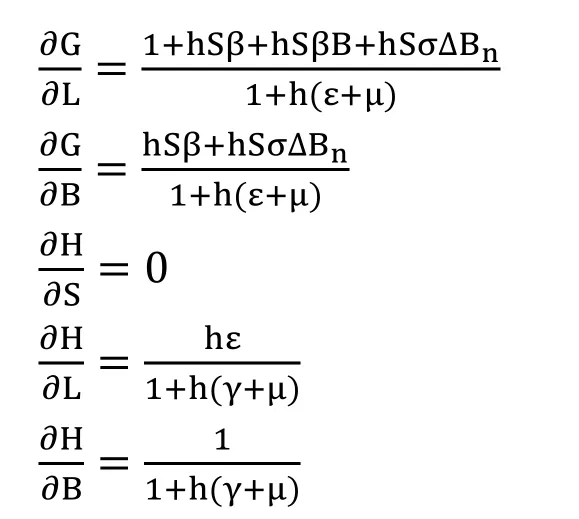
Now we want to linearize the model about the equilibria of the model for virus-free equilibrium V1=(S,L,B)=(1,0,0) and C∗＜1.

The given Jacobean is

The eigenvalues are

This is guaranteed to the fact that all eigenvalues of the Jacobean lie in the unit circle.So,the system (9) is LAS around V1.

4.5 Numerical trials

By using the values of parameters given in Yang et al.[Yang,Zhang,Li et al.(2012)],the numerical simulation is:

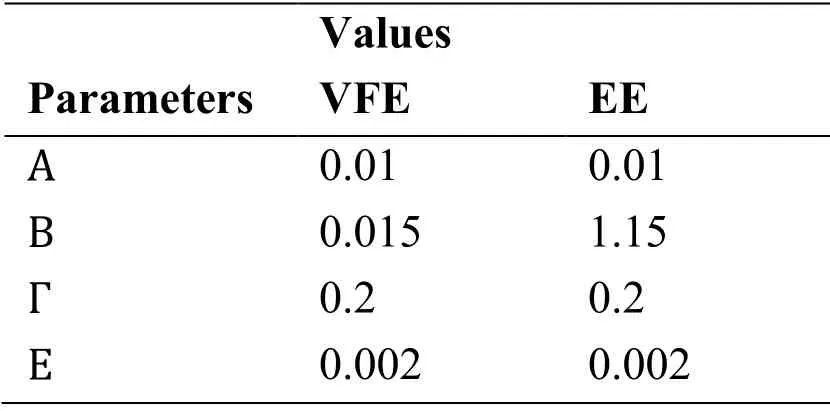
Table 2:Parameter values

M 0.5 0.5 σ 0.05 Estimated

4.5.1 Euler maruyama technique

The simulation for the system (5) is as follows:

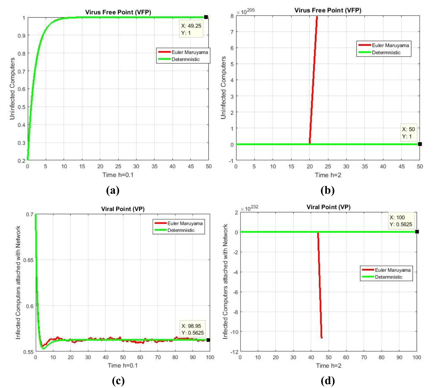
Figure 2:(a) Uninfected computers fraction for VFP at h=0.1 (b) Uninfected computers fraction for VFP at h=2 (c) Infected computers attached with network fraction for VP at h=0.1 (d) Infected computers attached with network fraction for VP at h=2

4.5.2 Stochastic euler technique

We pretend the solutions of the model (7) by utilizing Matlab database and parameters values assumed in Yang et al.[Yang,Zhang,Li et al.(2012)] (see Tab.2)

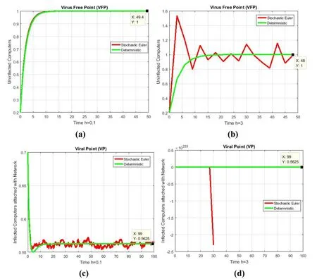
Figure 3:(a) Uninfected computers fraction for VFP at h=0.1 (b) Uninfected computers fraction for VFP at h=3 (c) Infected computers attached with network fraction for VP at h=0.1 (f) Infected computers attached with network fraction for VP at h=3

4.5.3 Stochastic runge kutta technique

We pretend the solutions of the model (8) by utilizing Matlab database and parameters values assumed in Yang et al.[Yang,Zhang,Li et al.(2012)] (see Tab.2)

Figure 4:(a) Uninfected computers fraction for VFP at h=0.1 (b) Uninfected computers fraction for VFP at h=4 (c) Infected computers attached with network fraction for VP at h=0.1 (d) Infected computers attached with network fraction for VP at h=4

4.5.4 Stochastic NSFD technique

We pretend the solutions of the model (9) by utilizing Matlab database and parameters values assumed in Yang et al.[Yang,Zhang,Li et al.(2012)] (see Tab.2)

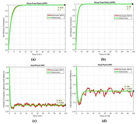
Figure 5:(a) Uninfected computers fraction for VFP at h=0.1 (b) Uninfected computers fraction for VFP at h=100 (c) Infected computers attached with network fraction for VP at h=0.1 (d) Infected computers attached with network fraction for VP at h=100

4.5.5 Comparison section

Comparison of explicit stochastic techniques with proposed SNSFD technique can be observed in this section as follows:

euler mayuyama and its average at h=2 (c) Spreader class with stochastic euler and its average at h=0.1 (d) Spreader class with stochastic euler and its average at h=3 (e) Spreader class with stochastic runge kutta and its average at h=0.1 (f) Spreader class with stochastic runge kutta and its average at h=4

4.5.6 Covariance of sub-populations

The covariance of different sub-populations of computer virus model has been discussed in this section.The outcomes of covariance of sub populations are as follows in Tab.3.

An inverse relationship can be seen between the uninfected class and the other two subpopulations.It shows that the increase in the uninfected class will occur with the decline in other sub-populations and ultimately the system attains virus-free equilibrium.

5 Outcomes and analysis

For discretisation parameter h=0.1,we see that euler maruyama technique meets to equilibria of the model,this can be seen by Fig.2(a) and Fig.2(c).On the other hand,the euler maruyama technique fails to sustain nonnegativity and even divergent,this can be seen by Fig.2(b) and Fig.2(d).For parameter h=0.1,we see that the stochastic euler technique meets to both equilibria,this can be seen by Fig.3(a) and Fig.3(c).On the other hand,for both equilibria the stochastic euler technique fails to maintain nonnegativity and consistency as shown in Fig.3(b) and Fig.3(d).For step size h=0.1,we see that the stochastic runge kutta technique converges to both equilibria,this can be seen graphically by Fig.4(a) and Fig.4(c).

The stochastic runge kutta technique fails to uphold stability and nonnegativity for both equilibrium points when we increase the step size this change happens in Fig.4(b) and Fig.4(d).Thus the aforementioned stochastic techniques do not sanctuary all the dynamical properties [Mickens (1994,2005)].On the other hand,for taking any discretisation parameter the stochastic NSFD technique converges for both equilibria,this can be seen by Fig.5.In Fig.6,we have presented the comparison of stochastic explicit and well-posed SNSFD techniques.

6 Conclusion and future framework

In comparison to deterministic computer virus model,the stochastic computer virus model is a more reliable strategy.The stochastic numerical techniques are detail-oriented and they work well for even minute time step size.They may lose the necessary properties of continuous dynamical system due to divergence on specific values of time step size.The SNSFD for computer virus model is capable of preserving important properties like positivity,dynamical consistency and boundedness.It is also appropriate for any time step size [Mickens (1994,2005)].For our future work,we are aiming to execute SNSFD to sophisticated stochastic delay and Spatio-temporal systems.Additionally,we could utilize the current numerical work in the extension of networking flows and fractional networking flows systems [Singh,Kumar and Baleanu (2019)].In future,we are going to work for the reaction diffusion and fractional-order stochastic computer virus models.

Acknowledgement:We are the greatful to Vice-Chancellor,Air Vice Marshal Faaiz Amir (Retd.),Air University,Islamabad for providing an excellent research environment and facilities.The third author also thanks Prince Sultan University for funding this work through research-group number RG-DES2017-01-17.

Declaration:All author(s) have no competation regarding about publication of this article.

References

Albazzaz,J.M.A.;Almuhanna,N.E.(2016).Avoiding computer viruses and malware threats.International Journal of Advanced Research in Computer and Communication Engineering,vol.5,no.11,pp.288-291.

Allen,E.J.;Allen,L.J.S.;Arciniega,A.;Greenwood,P.E.(2008):Construction of equivalent stochastic differential equation models.Stochastic Analysis and Applications,vol.26,no.2,pp.274-297.

Bayram,M.;Partal,T.;Buyukoz,G.O.(2018):Numerical methods for simulation of stochastic differential equations.Advances in Difference Equations,vol.17,no.5,pp.1466-1476.

Billings,L.;Spears,W.M.;Schwartz,I.B.(2002):A unified prediction of computer virus spread in connected networks.Physics Letters A,vol.297,no.3,pp.261-266.

Cai,L.;Li,X.Z.(2010):Global analysis of a vector-host epidemic model with nonlinear incidences.Applied Mathematics and Computation,vol.217,no.7,pp.3531-3541.

Cohen,F.(1987):Computer viruses.Computers and Security,vol.6,no.1,pp.22-35.

Fatima,U.;Ali,M.;Ahmed,N.;Rafiq,M.(2018):Numerical modeling of susceptible latent breaking-out quarantine computer virus epidemic dynamics.Heliyon,vol.5,no.5,pp.631-652.

Gard,T.C.(1988):Introduction to Stochastic Differential Equations.Marcel Dekker,New York.

Han,X.;Tan,Q.(2010):Dynamical behavior of computer virus on Internet.Applied Mathematics and Computation,vol.2,no.17,pp.2520-2526.

Karatzas,I.,Shreve,S.E.(1988):Brownian Motion and Stochastic Calculs.Springer-Verlag.

Karatzas,I.;Shreve,S.E.(1991):Brownian Motion and Stochastic Calculus,2nd Edition.Springer Verlag,Berlin.

Kloeden,P.E.;Platen,E.;Schurz,H.(1994):Numerical Solution of SDE Through Computer Experiments.Springer Verlag,Berlin.

Maruyama,G.(1955):Continuous markov processes and stochastic equations.Rendiconti Del Circolo Matematico Di Palermo,vol.4,no.1,pp.48-90.

Mickens,R.E.(1994):Nonstandard Finite Difference Models of Differential Equations.World Scientific,Singapore.

Mickens,R.E.(2005):A fundamental principle for constructing nonstandard finite difference schemes for differential equations.Journal of Difference Equations and Applications,vol.11,no.7,pp.645-653.

Mickens,R.E.(2005):Advances in Applications of Nonstandard Finite Difference Schemes.World Scientific,Singapore.

Mishra,B.K.;Jha,N.(2007):Fixed period of temporary immunity after run of antimalicious software on computer nodes.Applied Mathematics and Computation,vol.190,no.2,pp.1207-1212.

Murray,W.H.(1988):The application of epidemiology to computer viruses.Computers and Security,vol.7,no.2,pp.139-150.

Noeiaghdam,S.;Suleman,M.;Budak,H.(2018):Solving a modified nonlinear epidemiological model of computer viruses by homotopy analysis method.Mathematical Sciences,vol.12,no.3,pp.211-222.

Oksendal,B.(2003):Stochastic Differential Equations.Springer Verlag,Berlin.

Patil,B.V.;Jadhav,R.J.(2014).Computer virus and antivirus software a brief review.International Journal of Advances in Management and Economics,vol.4,no.2,pp.1-4.

Peng,M.;He,X.;Huang,J.;Dong,T.(2013):Modeling computer virus and its dynamics.Mathematical problems in Engineering,vol.1,no.6,pp.1-5.

Piqueira,J.R.C.;Araujo,V.O.(2009):A modified epidemiological model for computer viruses.Applied Mathematics and Computation,vol.2,no.13,pp.355-360.

Piqueira,J.R.C.;Vasconcelos,A.A.D.;Gabriel,C.E.C.J.;Araujo,V.O.(2008):Dynamic models for computer viruses.Computers and Security,vol.27,no.8,pp.355-359.Platen,E.(1991):An introduction to numerical methods for stochastic differential equations.Acta Numerica,vol.8,no.1,pp.197-246.

Raza,A.;Arif,M.S.;Rafiq,M.(2019).A reliable numerical analysis for stochastic dengue epidemic model with incubation period of virus.Advances in Difference Equations,vol.3,no.2,pp.1958-1977.

Ren,J.;Yang,X.;Yang,L.X.;Xu,Y.;Yang,F.(2012):A delayed computer virus propagation model and its dynamics.Chaos Soliton and Fractals,vol.45,no.1,pp.74-79.

Ren,J.;Yang,X.;Zhu,Q.;Yang,L.X.;Zhang,C.(2012):A novel computer virus model and its dynamics.Nonlinear Analysis Real World Applications,vol.13,no.1,pp.376-384.

Singh,J.;Kumar,D.;Baleanu,D.(2019):New aspects of fractional Biswas-Milovic model with mittag-leffer law.Mathematical Modeling of Natural Phenomena,vol.14,no.1,pp.303-319.

Wierman,J.C.;Marchette,D.J.(2004):Modeling computer virus prevalence with a susceptible infected susceptible model with reintroduction.Computational Statistics and Data Analysis,vol.45,no.1,pp.3-23.

Yang,L.X.;Yang,X.;Wen,L.;Liu,J.(2012):A novel computer virus propagation model and its dynamics.International Journal of Computer Mathematics,vol.89,no.17,pp.2307-2314.

Yang,L.X.;Yang,X.;Zhu,Q.;Wen,L.(2013):A computer virus model with graded cure rates.Nonlinear Analysis Real World Applications,vol.14,no.1,pp.414-422.

Yang,M.;Zhang,Z.;Li,Q.;Zhang,G.(2012):An SLBRS model with vertical transmission of computer virus over the Internet.Discrete Dynamics in Nature and Society,vol.20,no.12,pp.1-17.

Yao,Y.;Fu,Q.;Yang,W.;Wang,Y.;Sheng,C.(2018):An epidemic model of computer worms with time delay and variable infection rate.Security and Communication Networks,vol.2,no.1,pp.982-993.

Yu,Y.;Hu,J.;Zeng,Y.(2019):On computer virus spreading using node-based model with time-delayed intervention strategies.Science China Information Sciences,vol.62,no.5,pp.59201-59203.

Yuan,H.;Chen,G.(2008).Network virus epidemic model with the point to group information propagation.Applied Mathematics and Computation,vol.206,no.1,pp.357-367.

Zhang,C.(2018):Global behavior of a computer virus propagation model on multilayer networks.Security and Communication Networks,vol.1,no.1,pp.195-204.

Zhu,Q.;Yang,X.;Ren,J.(2012).Modeling and analysis of the spread of computer virus.Communication in Nonlinear Science and Numerical Simulation,vol.17,no.12,pp.5117-5124.