LQR Control of a Three Dimensional Underwater Glider

CAO Jun-jun,CAO Jun-liang,HU Yong-li,YAO Bao-heng,LIAN Lian

(The State Key Laboratory of Ocean Engineering,Shanghai Jiao Tong University,Shanghai 200241,China)

Abstract:This paper analyzes a linear system by simplification and linearization of the three dimensional system of underwater glider,and constructs a feedback control law to make the glider motion robust to the disturbances caused by inaccurate measurements or some other uncertain environments.The dynamic modeling of the system which governs buoyancy propelled,fixed wings underwater glider with internal moving mass is multi-input multi-output(MIMO),which is underactuated while easily affected by the ambient environment.A linear feedback control law is established to improve the control performance of the glider.Contrast results of simulations demonstrate that the derived LQR controller has faster response than Proportional Integral Derivative(PID),which manifests its outstanding capability in controlling the underwater gliders.

Key words:nonlinear system;linearization;simulation;underwater glider

0 Introduction

Nowadays,marine environmental information is the primary decision-making basis of marine exploitation,marine environmental protection,military affairs safeguard,oceanographic research and ocean administration.A vehicle called underwater glider is rapidly becoming important measuring apparatus in ocean sampling because of its high endurance and low cost.

To obtain oceanography data in real time with long-range,we need to ensure the safety of glider in complicated ocean environment.An accurate mathematical model should be established to analyze the operation of underwater glider.The mathematical model of glider by far can be divided into two main types-the general six-degree-freedom nonlinear equations of underwater vehicles by using the momentum theorem and theorem of moment of momentum,and the Lagrangian equations established from the kinetic energy perspective.

Today the widely used model of glider is a motion model derived by Leonard and Graver[1].Wang et al[2]established nonlinear dynamic equations based on Appell's equations,and Sun et al[3]built up a model by using the Kirchhoff equations and Newton-Euler method.

The greatest contributions in underwater glider control law have been made by Leonard,within which many methods are applied to a model of laboratory-scale underwater glider called ROGUE.The gliding path,motion stability and nonlinear control system[4]of the underwater glider[1],as well as the linear quadratic regulators and observer[5]of the motion in vertical plane,are also designed out and verified by test.Multi-gliders are studied to analyze cooperative control,adaptive sampling and motion stability[6].Graver analyzed the configuration and underwater movement properties of the glider systematically,and proposed a method using the acceleration of the internal moving mass as the input[1].Variable center of mass dynamic model of underwater glider is designed by Ge et al on the basis of which the simulation of the glider motion in the vertical plane is completed[7].Through the linearization and simplification of the dynamic model in vertical plane,the linear quadratic regulators are designed,and the performance of the regulator and system's ability to suppress interference and disturbance are analyzed[5].

The common points of the mentioned study are linear controlling area which is only limited in the vertical plane.Instead,the simplification and linearization of three dimensional models are developed in this paper,and the linear quadratic regulators control law to analyze the motion of the glider in spiraling is given.Compared with nonlinear control system,the linear control law is more convenient,and the traditional control theories can be used.The feedback control methodology designed in this paper can improve the currently applied glider control strategies in three dimensional spaces.

This paper is organized as follows：In Chapter 1,the model of glider is formulated and linearized;linear control law is derived in Chapter 2,and some simulation results of the controlled glider are presented;In Chapter 3,some conclusions and final remarks are given.

1 Glider dynamics

The dynamic equations for the underwater gliders used in this paper are presented in Ref.[8].The dynamic model of the glider is modeled as a rigid body(mrb)with fixed wings immersed in unbounded fluid,and with buoyancy control(mb)and internal moving mass(mp)which also can rotate around the x-axis.For simplicity,the center of the buoyancy is assumed to attach to the center of the rigid body.The entire coordinate frame of the system is shown in Fig.1.The origin of the body frame(B0-xyz)is fixed at the center of buoyancy and the inertial coordinate frame is fixed on the ground(E0-ijk).

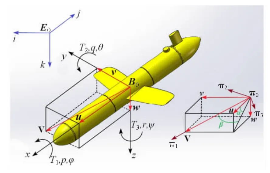
Fig.1 The coordinate frames

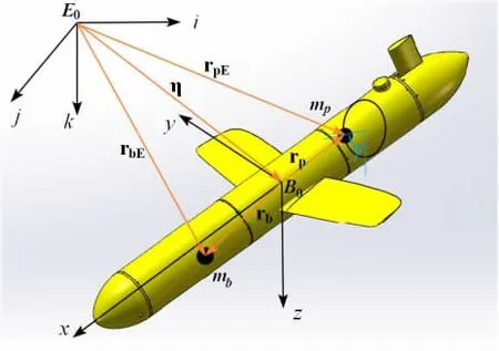
Fig.2 Some parameters defined of the glider

Let V=[u,v, w ]Tand Ω=[p,q,r]Tare the translational velocity and angular velocity of the glider respectively with respect to the body frame.Let η represents the position of the body frame origin with respect to the inertial frame,and then the vehicle kinematic equations are given by

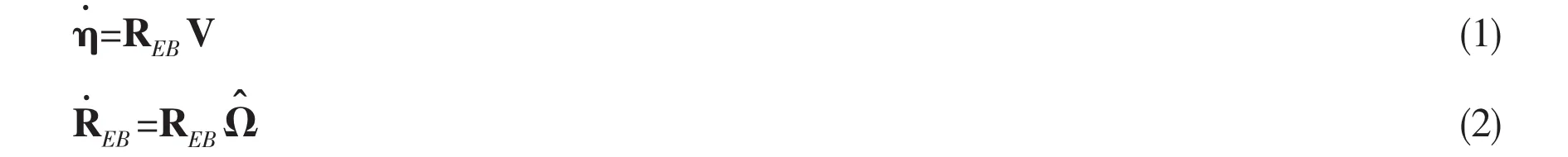
The rotation matrix REBis typically parameterized using the roll angle φ,pitch angle θ,and yaw angle ψ.The current coordinate frame(π0-π1π2π3)can be also translated to the body frame(B0-xyz)by using RBπ.The rotation matrix in the kinematic equations has previously been reported in Ref.[8].Let the characterdenote the 3×3 skew-symmetric matrix satisfying=a×b for 3-vectors a and b[1].

1.1 The nonlinear dynamic system

Through the Ref.[9],the dynamic equations of the glider can be presented as follows：

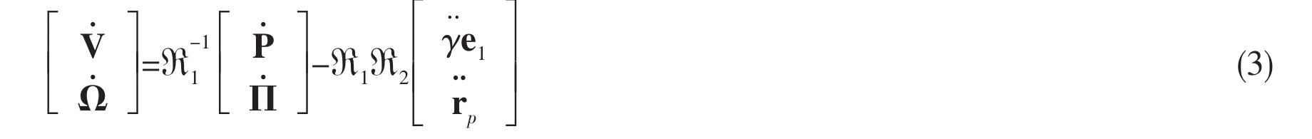
where ℜ1represents the inertial matrix of the vehicle/fluid system,ℜ2represents the inertial matrix of the internal moving mass.The inverse matrix is calculated out by using the method reported in Ref.[1].The P represents the total linear momentum and Π represents the total angular momentum of the vehicle/fluid system in body frame.Based on the theorem of momentum,the time derivative of P and Π can be written as following forms

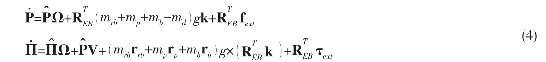
where fextand τextrepresent external forces and moments respectively.These forces and moments include viscous forces,such as lift and drag,and control moments,such as the yaw moment due to a rudder.In the current frame,The hydrodynamic force Fviscand moment Tviscare usually expressed as：

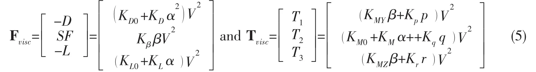
where D represents the drag force,SF represents the slip force,L the lift force,and α and β represents the attack angle and the slip angle,respectively,i.e.tanα=w/u,tanβ=v/sqrt（u2+w2）.The external force fextand moment τextcan be shown as follows：

1.2 Simplification of the nonlinear system

Summarizing above equations,a group of complex equations includes mass nonlinear and coupling terms can be derived out.With these terms,it is difficult to obtain steady state results of rp1d,mbdand γd,whatever analytical methods or numerical methods are used.In this section,by using some approximations,the nonlinear system is simplified with following properties：

(1)When the glider is under stable sliding state,the equilibrium values of vd,wd,pd,qdand rdare small,and the influence of coupling terms with them is extremely limited to the kinematic equations,so the coupling terms including vd,wd,pd,qdand rdcan be ignored,where the subscript d denotes the value of all variables at the glide equilibrium;

(2)In spiraling equilibrium state,compared with the value of u,v and w usually are very small,so Vd≈ud,cosαd≈1,sinαd≈wd/ud,cosβd≈1,sinβd≈vd/ud;

(3)The values of αdand βdare usually small in stable state,which can be simplified by using the first-order Taylor expansion αd≈sinαd,βd≈sinβd.

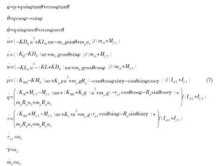
Then the nonlinear system can be simplified as Eq.(7).

1.3 Linearization

Spiraling motion is an important motion of the glider for position or turning.In this section,the linearization is determined for three dimensional gliders with steady spiral gliding.When the glider is spiraling,the heading angle ψ is always changed,and the time derivation of it is constant.Ψ can be calculated out easily by using other equilibrium values.

Here,let x= （φ,θ,u,v,w,p,q,r,rp1,γ,mb）Tand u=（u1, u2,u3）T,and define δx=x-xdand δu=u-ud.Then the linearized system is shown as follows：

where A and B are defined as：

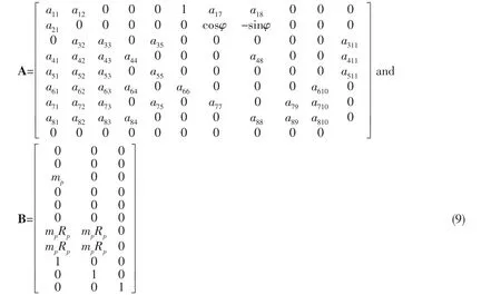
The abbreviated items are shown as follows：

Compared with nonlinear systems,the linear system designed above is able to test the design parameters of a vehicle easily,and then all classical control theories can be applied to the glider systems.The system can be helpful to analyze the stability and controllability of underwater gliders in three dimension space.A is a constant matrix when the glider is in steady state,and it reflects the inherent performance of the glider.Through the sensors the three inputs can be obtained,and then the given state variables can be simulated or computed with time according to Ref.(8).

2 Feedback control

For past few years,underwater gliders had been used in many fields,such as deep-sea explorations,the inspections and tracking of hydrothermal sources,and so on.When gliders carry out the tasks,spiraling or turning motions to adjust the attitudes are required.In this chapter the spiraling motion of glider is mainly focused on.The glider is considered to be spiral downwards,by starting a downward steady gliding and then using a linear feedback controller to drive it to another steady gliding.

The LQR(linear quadratic regulator)method is used to design the linearization controller.This standard linear control method generates a stabilizing control law which needs the cost function is minimum.The cost function is a weighted sum of the squares of the states and the input variables,which is defined as follows：

where Q and R are state penalty matrix and control penalty matrix,respectively.They are cho-sen to prevent large motions about the internal moving mass and variable mass when the glider would change the attitudes or face some disturbances.They can arrange the mass motion in the physical limitations,and the values of Q and R with this consideration provide

The four matrixes(A,B,Q,R)of the Riccati equation are all produced.MATLAB is used to solve the equation and obtain the control gain K.Then the corresponding control law can be computed.

3 Simulation results

To verify that the approximate system is similar to the original full system,we compared the simulations results of two systems by using PID control.The parameters applied in this study are given in Ref.[10]and listed as follows：mrb=54.28 kg,mp=11 kg,mb=(-0.5 kg,0.5 kg),Mf1=1.48 kg,Mf2=49.58 kg,Mf3=65.92 kg,If1=0.53 kg·m2,If2=7.88 kg·m2,If3=10.18 kg·m2,KD0=7.19 kg/m,KD=386.29 kg/m/rad2,KL0=-0.36 kg/m,KL=440.99 kg/m/rad,KM0=0.28 kg,KM=-65.84 kg/rad,Kp=-19.83 kg·s/rad2,Kq=-205.64 kg·s/rad2,Kr=-389.30 kg·s/rad2.The values of rp1,γ,and mbcan be measured out by the sensors equipped on the glider.The three parameters are used to be input variables of the system,and both of systems are simulated to get the change curves of the state variables.The feedforward control function in this case is chosen as：

In Fig.3,a period of glider motion from γ=5.73°to γ=37.24°downward spiraling is shown,while the position of movable mass rp1is 5.5 mm and the ballast mass mbis 0.33 kg.The pa-rameters of the PID control method are KP=-0.5,KI=-0.15,KD=-0.67.Tab.1 also gives other simulation results of key variables for various input parameters.

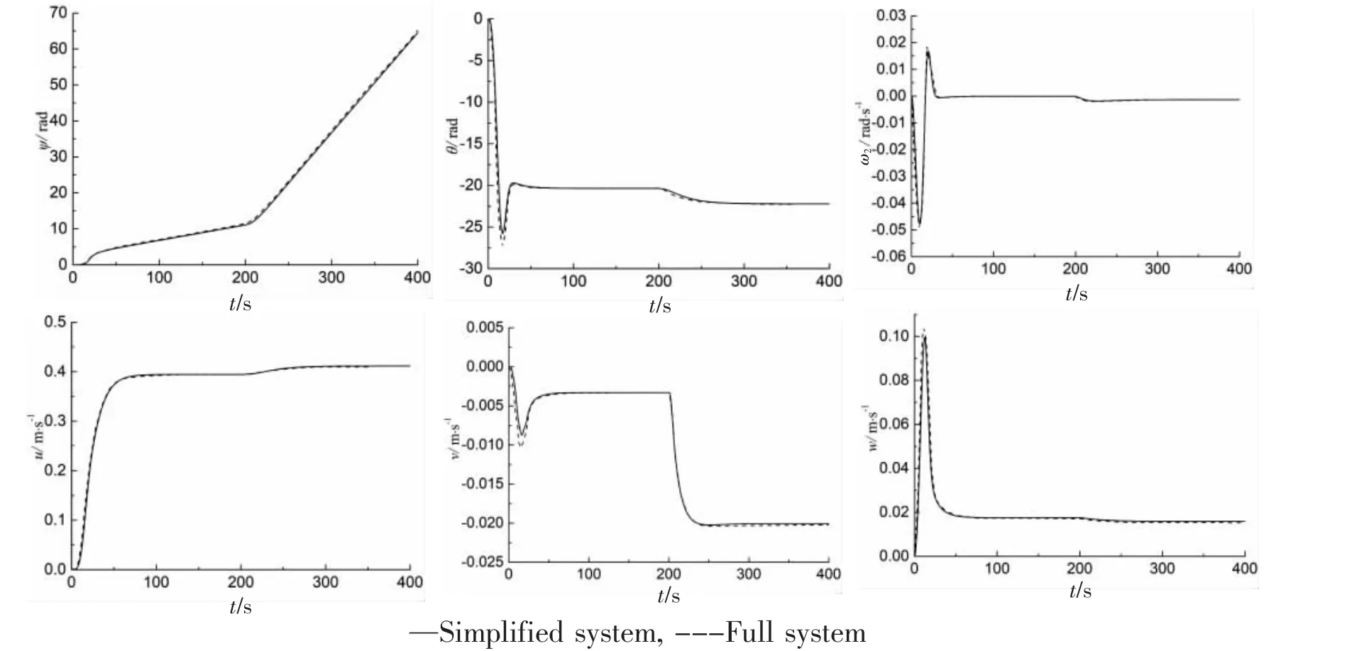
Fig.3 Output responses of glider dynamics by using PID control

Tab.1 Comparison of approximate and actual steady motion parameters

Fig.4 Output responses of glider dynamics with LQR control and PID control

From the comparison of the simplified and full system of the glider,the simplified dynamic system was used to analyze the LQR control method.Fig.4 is the comparison responses of simplified system by using LQR and PID control method.Let the glider spiral downward with the internal mass rotate angle γ=5.73°and the variable mass mb=0.33 kg,the rotate angle is changed to 37.24°,the variable mass to 0.43 kg at t=200 s.The parameters of the PID control method are KP=-0.6,KI=-0.25,KD=-0.57.

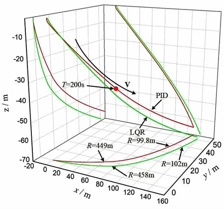
Fig.5 Comparison of path between PID control and LQR control

From the comparison of output responses of the two control methods(Fig.4),the LQR control method has faster response than the PID control method,while the tra-jectory at the switching stage has small fluctuation which is not much affecting the gliding motion of the glider.The gliding paths of the two methods are shown in Fig.5.Therefor the LQR control method has a better control performance than PID control.

4 Conclusion

In this paper,LQR control law has been derived out and applied to analyze the glider system that is established by simplifying and linearization the three dimensional system of the underwater glider.The system of the gliders is characterized by underactuation,high dimensionality,nonlinearity and coupling,which all make glider difficult to maneuver.Therefore,we rewrite the dynamic system by simplifying and linearization,the system was transformed into a linear system.Through the simulation results,it is demonstrated that the approximate linear system can replace the general nonlinear system.Based on the linear system,a feedback control law is developed to control the motion of underwater glider.The contrast results of simulations have demonstrated that the derived LQR controller has faster response than PID control methods.

In future work,some experiments are required to verify the results described in this paper.Some advanced control methods,by using adaptive control and sliding mode control are under development.