Practical BRDF reconstruction using reliable geometric regions from multi-view stereo
2019-02-27TaishiOnoHiroyukiKuboKenichiroTanakaTakuyaFunatomiandYasuhiroMukaigawa
Taishi Ono, Hiroyuki Kubo(), Kenichiro Tanaka, Takuya Funatomi, and Yasuhiro Mukaigawa
Abstract In this paper,we present a practical method for reconstructing the bidirectional reflectance distribution function (BRDF) from multiple images of a real object composed of a homogeneous material. The key idea is that the BRDF can be sampled after geometry estimation using multi-view stereo (MVS) techniques.Our contribution is selection of reliable samples of lighting, surface normal, and viewing directions for robustness against estimation errors of MVS. Our method is quantitatively evaluated using synthesized images and its effectiveness is shown via real-world experiments.
Keywords BRDF reconstruction; multi-view stereo(MVS); photogrammetry; rendering
1 Introduction
The reconstruction of three-dimensional (3D) shapes from multi-view images,generally known as the multiview stereo (MVS) technique, has been extensively studied [1]. MVS techniques generally ignore the bidirectional reflectance distribution function(BRDF)even though it is important for photo-realistic computer graphics. Our goal is to develop a BRDF estimation method that is suitable for the existing MVS pipeline with minimal additional observations.To make our method compatible with any MVS method, our method only relies on the output of MVS①Here, we demonstrate results based on 3D reconstruction using Agisoft PhotoScan, a commercial software package widely used in cinema and game studios..
To recover the BRDF, multiple pairs of lighting and viewing directions are required. The key idea is that a huge number of pairs can be acquired from an image captured under a single light source if the target object is homogeneous. Hence, the BRDF is recoverable even from a few images. If the lighting is known, then the BRDF is easily sampled because the viewing angle and surface normal may be obtained by MVS techniques.
The major challenge of this work is how to manage the estimation errors of the MVS algorithm. Because MVS algorithms generally assume that surfaces reflect diffusely, the reconstructed 3D shape includes errors caused by the rich BRDF. Even though the shape error is small, the surface normal is easily distorted,particularly when the reconstructed mesh is finely detailed. Although the error in the surface normal could be effectively reduced if we could integrate photometric stereo techniques such as Ref. [2], this is not desirable because it requires observations under additional light sources. The error in the normal affects the BRDF estimate. Thus, we introduce three physically-based criteria to select reliable pairs to robustly estimate the BRDF. After selecting reliable pairs, a parametric BRDF can be recovered by Nielsen et al.’s method [3]. Although this approach assumes a homogeneous object, it can be extended to heterogeneous objects using a simple method, where regions of the same material are manually segmented in each image and the method is applied to each material separately. The effectiveness of this method is shown via synthetic and real-world experiments.
2 Related work
There have been numerous studies on reconstructing the geometry of an object from multi-view images, a field known as MVS [1]. Many MVS algorithms [4—6]work poorly for non-Lambertian surfaces because the captured images are the result of complicated interactions between geometry, lighting, and material reflectance.
Some early studies considered mirror reflection [7,8]. To handle the behavior of general non-Lambertian materials Furukawa and Ponce [9] evaluated the photometric constancy and simply ignored images with bad scores. Treuille et al. [10] used reference images captured using known geometry, and under the same lighting and camera conditions as the target object. Chandraker et al. [11] correctly modeled the dependence of image formation on BRDF and illumination. Under perspective projection, they showed that four differential motions are sufficient to constrain the shape, even when the BRDF and illumination are unknown, using an invariant relating surface depth to image derivatives. In Ref. [12],Chandraker extended his theory of object motion to camera motion. He showed that three differential camera motions suffice for an unknown isotropic BRDF and unknown directional lighting. Li et al. [13] developed a robust BRDF-invariant shape reconstruction technique that requires only a single light field image. They formulated a general energy function composed of a texture gradient term and BRDF-invariant term, and then minimized this function to reconstruct the object’s surface. As exemplified above, many MVS techniques have been proposed to make reconstruction robust for a non-Lambertian target.
To reconstruct the 3D shape and BRDF from a real object, Schwartz and Klein [14] constructed a domeshaped device composed of 11 cameras,198 LED light sources, and 4 projectors. They captured more than 186,000 images using a turntable, and reconstructed the polygonal mesh and bidirectional texture function.Xia et al. [15] estimated both the spatially varying surface reflectance and detailed geometry from a video of a rotating object underunknown static illumination.They decoupled reflectance and normal reconstruction from geometry reconstruction, and formulated an iterative process to acquire detailed results. Oxholm and Nishino [16] estimated the reflectance and geometry under known but uncontrolled natural illumination by solving the likelihood representation with a few priors. However, they require special devices or complex conditions. Thus, the method’s practicability remains uncertain.
The BRDF characterizes material appearance, so BRDF reconstruction from a real object is of great importance in photorealistic computer graphics. A gonioreflectometer directly samples the BRDF for all lighting and viewing directions [17]. Miyashita et al. [18] proposed a rapid reconstruction method for spatially varying BRDFs using a projector,high-speed camera, and LEDs. This approach requires special devices, so is less practical than our method which requires only an ordinary camera and illumination.
Using a homogeneous sphere or cylinder, an isotropic BRDF can be recovered from an image [19].Nielsen et al. [3] significantly reduced the number of samples for BRDF reconstruction of a sphere. They extracted the principal components of the set of BRDFs from the MERL BRDF database [20] and optimized the sampling directions to minimize the condition number of the related acquisition matrix.We extend these ideas to an arbitrary shape using MVS reconstruction. In this paper, we propose a practical technique for BRDF reconstruction from real objects using multi-view images and a few additional images for acquiring the reflectance.
3 BRDF reconstruction from multi-view images
The BRDF is a four-dimensional quantity defined by lighting and viewing directions, but this can be reduced to a 3D form under the general assumption that the BRDF is isotropic. In this paper, we always make this assumption.
To reconstruct the BRDF,it is necessary to sample the reflectance from various pairs of lighting and viewing directions. After reconstructing the geometry from multi-view images, we can acquire the surface normal of the target object and the viewpoints of the input images, as shown in Fig. 1. Thus, if we know the illumination conditions of the input images, we can sample the reflectance using these lighting and viewing directions. However, multiview images for MVS are typically captured under ambient lighting, as shown in Fig. 2(a); in such cases, the illumination is complicated. To easily sample the reflectance, we prepare a few additional images captured under a distant light to acquire the reflectance (see Fig. 2(b)). Consequently, we can acquire the lighting and viewing directions for each pixel, and then sample the reflectance from every illuminated pixel in these distant light images.
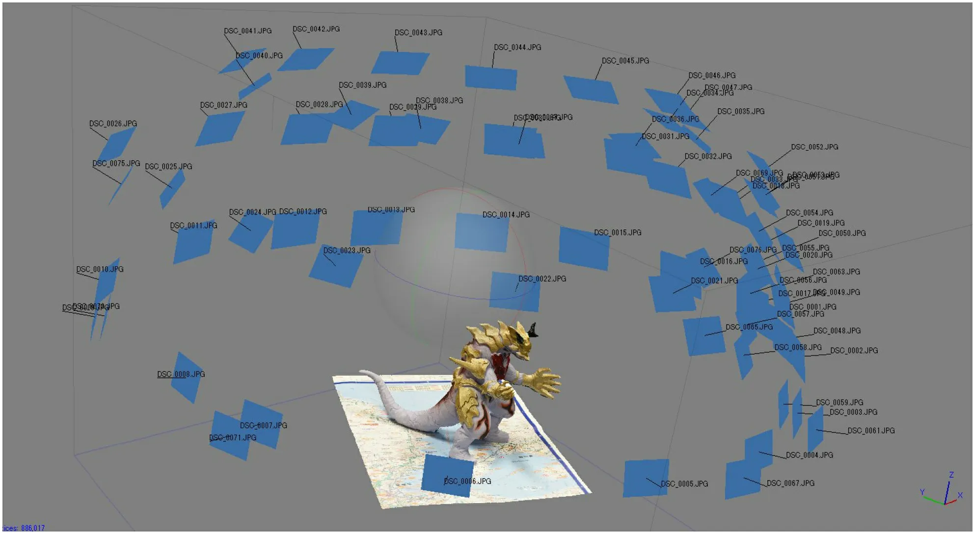
Fig. 1 Geometry reconstruction result using commercial software PhotoScan. Each blue square represents the estimated viewpoint of the input images.
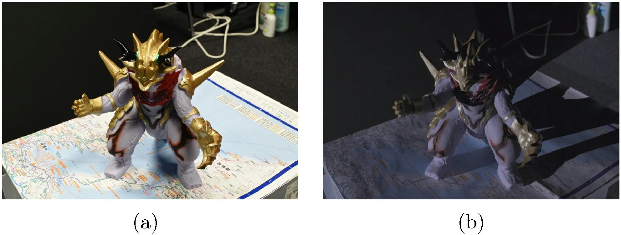
Fig. 2 (a) Example of the multi-view images with ambient lighting for acquiring geometry. (b) Example of a few additional images with one distant light for acquiring reflectance. Note that (a) and (b) were captured from the same viewpoint.
A naive approach requires hundreds of distant light images to be acquired because we must prepare millions of lighting and viewing directions for BRDF reconstruction. Preparing hundreds of such images is very inconvenient; so instead, we use an analytic method to reconstruct the BRDF from only a few samples [3]. This method reduces the number of samples using the principal components of BRDFs.
The procedure is as follows. First, we capture the multi-view images under ambient lighting to acquire the geometry and a few additional images under a single distant light to acquire the reflectance. Note that these distant light images share a viewpoint with one of the corresponding multi-view images, as shown in Fig. 2(a) and Fig. 2(b). The geometry is reconstructed from the multi-view images, and then the lighting and viewing directions are determined for all illuminated pixels in the distant light images. Next,using the acquired lighting and viewing directions,we determine the optimal lighting and viewing directions in accordance with Nielsen et al.’s method [3] and calculate the reflectance at the corresponding pixels of the distant light images. Finally, we reconstruct the BRDF using these optimal samples. Figure 3 overviews our method.
3.1 Estimating the BRDF from a few samples
We next briefly review how to reconstruct the BRDF from five optimal samples [3]. First, the principal components are extracted from measured BRDFs [20]. They are measured in a 3D volume using Rusinkiewicz’s half-difference angle coordinates(θh,θd,φd) [21]. The resolution in this volume is 90°×90°×180°=1,458,000 samples.
LetX ∈Rm×pdenote the matrix of all MERL BRDF observations, where the rows correspond to the mapped BRDFs and the columns correspond to particular lighting and viewing directions. In this case,m= 300 BRDFs are available, andp=1,458,000. The matrix of principal componentsQ ∈Rp×kis acquired by performing singular value decomposition after subtracting the mean BRDF:

The BRDFxis represented using a linear combination of the principal components:

Upon observingnsamples,each observationcan be written as follows:

In our method, to use the acquired lighting and viewing directions, we find the optimal lighting and viewing directions that minimize this condition number. We define the optimal samples as the corresponding reflectances of the distant light images.
4 Reliable region extraction

Fig. 3 Overview of our method. First, we obtain multi-view images under ambient lighting to acquire the geometry. We then obtain a few additional images with only one distant light to acquire the reflectance. Note that these distant light images share a viewpoint with one of the corresponding multi-view images. Next, we reconstruct the geometry using PhotoScan. We then extract reliable regions from the reconstructed geometry following assumptions introduced in this paper. Nielsen et al.’s optimal lighting and viewing directions are determined using the acquired lighting and viewing directions, and the reflectance is sampled at corresponding pixels of the distant light images. Finally, we reconstruct the BRDF using these samples.
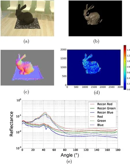
Fig. 4 (a) Example image captured with ambient lighting, for acquiring geometry. (b) Example image captured with a distant light, for acquiring reflectance. (c) Reconstructed normal map using PhotoScan. (d) Error map (in radian) of the angle between the reconstructed surface normal and ground truth. (e) Comparison to the ground truth (dashed line) of reconstructed BRDFs without considering surface normal error (solid line).
Although the MVS algorithm relaxes the Lambertian assumption, the reconstructed geometry includes estimation errors, particularly for non-Lambertian surfaces. Figure 4 shows how the reconstructed surface is distorted if the surface is non-Lambertian,via an example. Thus,the BRDF cannot be estimated correctly because of the unreliability of the estimated lighting, normal, and viewing directions. Figure 4(e)shows variation in BRDF values on the slice of incident light at 135°. Close to 45°, which represents specular reflection, we can observe a significant difference between the reconstruction (solid line) and ground truth(dashed line). This is because the errors in the normal direction prevent us from sampling the reflectance accurately.
4.1 Assumptions for extracting reliable regions
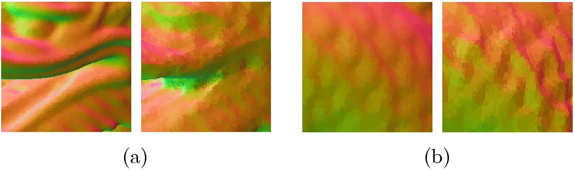
It is possible to improve the BRDF reconstruction accuracy by only using reliable regions; that is, we ignore unreliable regions in the MSV results when reconstructing the BRDF. To do so, we introduce three assumptions for extracting reliable regions from the reconstructed geometry. First,we assume that the estimation error is correlated with the curvature of the geometry,because the estimated geometry tends to be blurry(Fig.5(a))or bumpy(Fig.5(b)). Therefore,we assume that the surface normal directions in regions of higher curvature are unreliable. Second,we assume that the reflectance distribution is monotonic with respect to the cosine of the angle between the surface normal and the half vector. This assumption was originally introduced by Higo et al. [22]. Finally,regarding the distant light images, we also assume that the region of highest intensity represents the peak of specular reflection.
In our method, we implement these assumptions as constraints using the following steps.
Curvature.First, we acquire the curvature about each pixel of the distant light images using the method of Vergne et al. [23]. Let→p=(nx,ny,nz) denote thenormal direction at pointpin image space. We calculate the curvatureHas follows:
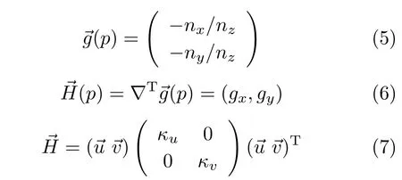
We useH= (κu+κv)/2 as the curvature of each pixel.
First,we compute the reconstructed surface normal(Fig. 6(a)) and the curvature about each pixel(Fig. 6(b)). We then remove unreliable pixels having higher curvature than a threshold. Figure 6(c) shows an example of the resulting mask, in which white pixels are excluded.
Monotonicity of reflectance.Given lighting directionviewing directionsurface normaland half vectorwe assume that the BRDFrat different pixelsiandjsatisfies the following:

in other words, as the dot product of surface normaland half vectorincreases, the BRDFralso increases.
We calculate this dot product and reflectance for all optimal samples, and continue to find optimal samples until all chosen samples satisfy Eq. (8).
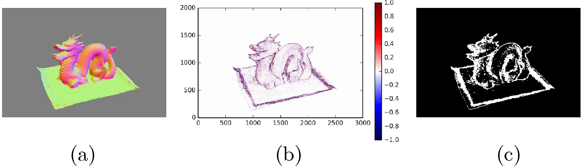
Fig.6 (a)Reconstructed surface normal map. (b)Acquired curvature.(c) Mask using the threshold.
Region with highest intensity.For the regionkwith highest intensity, we assume that the directions of half vectorand surface normalare equal:

or in other words, the intensity observed in regionkis due to a specular reflection.
We determine the pixel with the highest intensity among all pixels in the distant light images and then modify its surface normal to satisfy Eq. (9).In choosing the optimal samples, we minimize the condition number, while ensuring this modified pixel is included.
4.2 Random reconstruction and selection of most plausible result
Even after extracting the reliable regions, there will still be some errors in the surface normal directions.Therefore,to acquire a plausible result,we reconstruct several BRDFs using the reliable regions and choose the best reconstructed BRDF from these results.
First, we randomly select a number of these reliable regions,and acquire optimal samples using the randomly chosen regions. Then,we reconstruct several plausible BRDFs from different optimal samples.
Next, we select the best reconstruction result from these BRDFs. The best reconstruction is determined by comparing the intensity distribution between the distant light images (Fig. 7(a)) and reconstructed images (Fig. 7(b)). We render the images using the reconstructed BRDF and reconstructed geometry, as shown in Fig. 7(b). Note that these reconstructed images are rendered from the same viewpoint as one of the distant light images. We then acquire the intensity distributionsA=(a1,...,an),B=(b1,...,bn): see Fig. 7(a) and Fig. 7(b). Next, we calculate their cosine similarity cosand define the best BRDF as the one with maximum cosine similarity.
5 Experiment using simulated data
We conducted an experiment on simulated data using the MERL BRDF database (six BRDFs) and the fully measured geometry (Stanford BunnyandDragondistributed by Stanford Computer Graphics Laboratory) as the ground truth.
5.1 Experimental environment
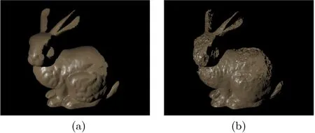
Fig. 7 (a) Example distant light image. (b) Example rendered image using the reconstructed BRDF and reconstructed geometry.Comparing the intensity distribution in (a) and (b) allows us to determine the best reconstructed BRDF.
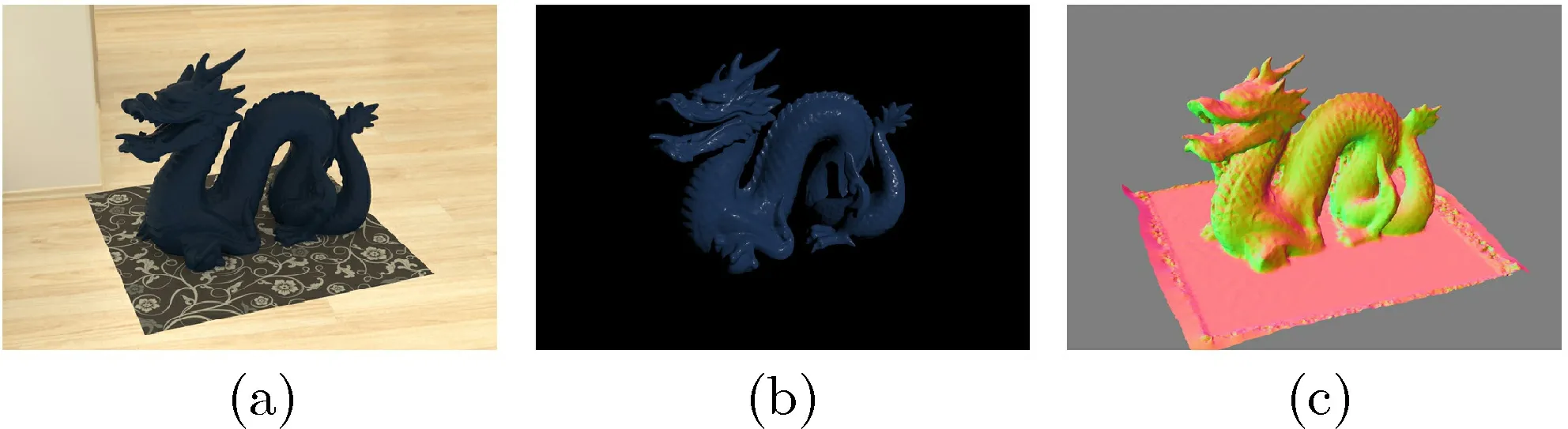
Fig. 8 Simulated example with blue-acrylic BRDF and Dragon geometry. (a) Example multi-view image with ambient lighting,for acquiring geometry. (b) Example single distant light image, for acquiring reflectance distribution. (c) Surface normal map acquired from multi-view images.
Figure 8(a) shows an example of the rendered multiview images with ambient lighting for acquiring geometry. In this case we rendered 72 images with resolution 3000×2000 pixels usingpbrt[24]. These images covered a sphere around the target object.Figure 8(b) shows an example of the images rendered with a virtual single distant light. These images were used to calculate the BRDF at chosen pixels. In this case, we used eight images for BRDF reconstruction.Each distant light image was rendered from the same viewpoint as one of the 72 multi-view images, and these eight viewpoints were determined arbitrarily,ensuring that the specular peak was contained. For 3D reconstruction, we usedAgisoft PhotoScan, a widely used commercial software package. Note that the estimation error in the reconstructed geometry is naturally included because the MVS algorithm is not perfect. In this case, we set the curvature threshold to 0.2 and used six optimal samples for BRDF reconstruction. In this experiment, we randomly reconstructed 10 BRDFs and chose the best BRDF as described in Section 4.2.
5.2 Experimental results
Figure 9 shows the resulting reconstructed BRDFs.The graphs on the left compare the reconstructed BRDFs (solid line) to the ground truth (dashed line).These graphs represent the reflectance transition as the viewing direction varies from 0 to 180°. In all graphs, the surface normal, lighting, and viewing directions are located in the same plane, and the lighting direction is at 135°. In comparison with Fig. 4(e), we can observe a noticeable improvement in reconstruction quality, in particular near 45°,which represents the specular reflection. From these graphs, we can conclude that the extracted reliable regions provide plausible optimal samples for BRDF reconstruction.
However, in the experiment usingfruitwood-241andStanford Bunny(the second from the top of Fig. 9), the shape of the reconstructed BRDF is slightly different to the ground truth. In our method,the specular peak can be accurately reconstructed using the highest intensity assumption. However,when the BRDFs vary gradually, the reconstruction error tends to be large. Our reconstructed results have a sharper shape than the ground truth because some surface normal errors persist. Additionally,with flatter BRDFs, such aspink-fabric(third),pinkfabric2(fifth), andgreen-latex(sixth), the highest intensity assumption causes the reconstructed results to have a small specular peak, which is not observed in the ground truth.
The pictures on the right show spheres rendered using the reconstructed BRDFs (lower) and ground truth (upper). In terms of color and specularity,the reconstructed BRDFs are quite similar to the ground truth. Additionally,regarding the flat BRDFs,the small specular peaks do not influence their appearance. These images indicate that the results using our method have a plausible appearance.
5.3 Evaluation of each assumption
We now evaluate the effectiveness of each assumption.Figure 10 shows evaluation results from two simulated examples using theStanford Bunnywithblue-acrylicand theDragonwithalum-bronze.
The upper two graphs represent the summed reconstruction error:

over all lighting and viewing directions. We randomly reconstructed the BRDF several times using each assumption and computed the mean and standard deviation of the reconstruction error. From the left,each bar represents the reconstruction result (i)without any assumptions,(ii)using only the curvature assumption, (iii) using only the monotonicity assumption, (iv) using only the highest intensity assumption,and(v)using all assumptions. Compared to the result using no assumptions, we can observe that the reconstruction error decreases with each assumption. Case(i)can be considered to correspond to Ref. [3].
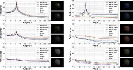
Fig. 9 Reconstructed BRDFs for alum-bronze, fruitwood-241, pink-fabric, blue-acrylic, pink-fabric2, and green-latex from the MERL BRDF database. Each graph compares the reconstructed BRDF (solid line) to the ground truth (dashed line). Each line represents the transition in the BRDF value when the incident light is at 135° and the viewpoint is located on the same plane as the incident light. The rendered sphere images have a front light at [1,1,1] and a back light at [-1,-1,3]. Above: rendered using ground truth. Below: rendered using reconstructed BRDFs.
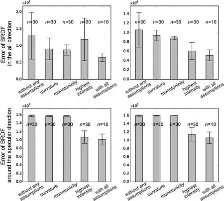
Fig. 10 Mean and standard deviation of BRDF reconstruction error.Above: calculated reconstruction error for all lighting and viewing directions. Left to right: reconstruction result without assumptions,using only the curvature assumption, using only the monotonicity assumption, using only the highest intensity assumption, and using all assumptions. Below: reconstruction error around the specular direction.
The lower two graphs show the reconstruction error in the specular reflection, as this has a considerable influence on appearance. From these graphs,it is clear that the highest intensity assumption significantly reduces the reconstruction error in the specular reflection.
From these evaluations, we can conclude that each assumption reduces the reconstruction error, and we can acquire the most plausible result using all assumptions: the assumptions complement each other to improve the estimation.
5.4 Correlation between intensity distribution and BRDF reconstruction error
To evaluate the effectiveness of the random sampling described in Section 4.2, we randomly reconstructed the BRDF 10 times for each simulation. For every reconstructed BRDF, we rendered the reconstructed images and acquired the cosine similarity with the distant light images. Figure 11 shows the correlation between the cosine similarity and the BRDF reconstruction error. These graphs indicate that,in most cases, the highest cosine similarity result provided one of the smallest reconstruction errors.
However, in the experiment withpink-fabric(Fig.11(lower right)), this approach gave the seventhbest error. This is partly because BRDFs with low viewpoint dependency do not produce a characteristic intensity distribution. For diffuse-like BRDFs, this approach does not work well.
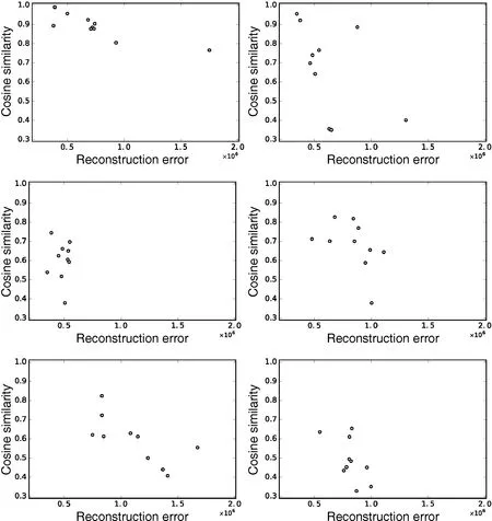
Fig. 11 In a simulation, we reconstructed the BRDF 10 times and computed the correlation between the cosine similarity and the BRDF reconstruction error. The graphs represent cases using Dragon withalum-bronze (upper left), Stanford Bunny with blue-acrylic (upper right), Dragon with green-latex (middle left), Stanford Bunny withfruitwood-241 (middle right), Dragon with pink-fabric2 (lower left),and Dragon with pink-fabric (lower right).
6 Experiments using real data
In this section, we present the results of several experiments using real data to show the practicability and effectiveness of our method.
6.1 Indoors experiments
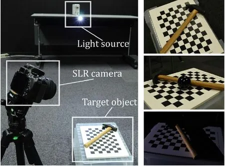
Fig. 12 Left: experimental setup. Upper right: example multiview image with room lighting for acquiring geometry. Middle right:picture with a glossy black sphere for obtaining the light direction.Lower right: example distant light image for acquiring the reflectance distribution with a single distant light.
Hammer.We first reconstructed the BRDF of a hammer. The experimental setup is shown in Fig. 12(left). We used a Nikon D5500 SLR camera to capture images and a SIGMAKOKI SLA-100A as the distant light. We obtained 73 multi-view images with room lighting to acquire the geometry(Fig. 12(upper right)) and eight images with distant light (Fig. 12(lower right)). We overlapped each multi-view image by at least 60%, and moved the camera manually to capture the images. All images were captured with a resolution of 6000×4000 and a fixed focal length. To determine the light direction and intensity in the distant light images,we used a glossy black sphere (Fig. 12(middle right))and a white reflector. In this experiment, we considered the hammer to be composed of two materials,so we separately reconstructed the BRDF of the hammer’s head and body using hand-made mask images (Fig. 13(b)). In all experiments using real data, we set the curvature threshold to 0.2, randomly reconstructed 10 BRDFs, and used six optimal samples for BRDF reconstruction.
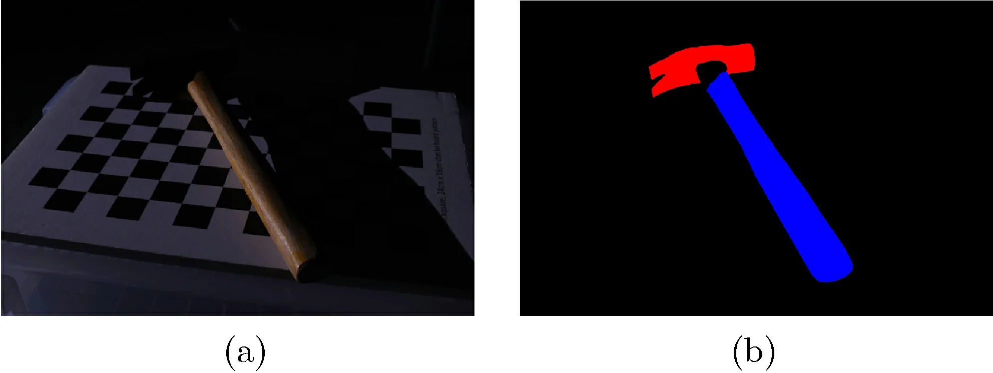
Fig. 13 (a) Example distant light image. (b) Example mask image used to acquire the reflectance individually from the hammer’s head and body. These mask images were constructed for each distant light image.
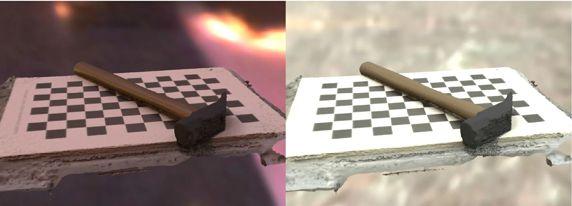
Fig. 14 Rendered images using the reconstructed BRDF with two lighting environments (Grace Cathedral (left) and Eucalyptus Grove(right), Paul Debevec 1998, 1999).
Figure 14 shows images rendered with the reconstructed BRDF from the head and body of the hammer. In Fig. 14, the reconstruction of the hammer’s glossy body and matt head is plausible.Ideally, several BRDFs must be assumed for the hammer’s body because it is made of wood. To acquire a more plausible appearance,it is necessary to consider another approach to separate the materials rather than hand-made mask images (Fig. 13(b)).This problem remains as future work.
Kaiju figure.Next, we reconstructed the BRDF of thekaijufigure shown in Fig. 15(a). We input 67 multi-view images to acquire the geometry and eight distant light images to acquire the reflectance(Fig. 15(b)). We excluded the cast shadow using the mask images shown in Fig. 15(c). In this case, we automatically formed these images using the reconstructed geometry and estimated lighting direction. We separated this figure into a gold part(blue area in Fig.15(d)),black horn part(yellow area),black line part (green area), purple body part (white area), and red chest part (red area), and individually reconstructed five BRDFs using the mask images(Fig. 15(d)). Again, we constructed the mask images manually.
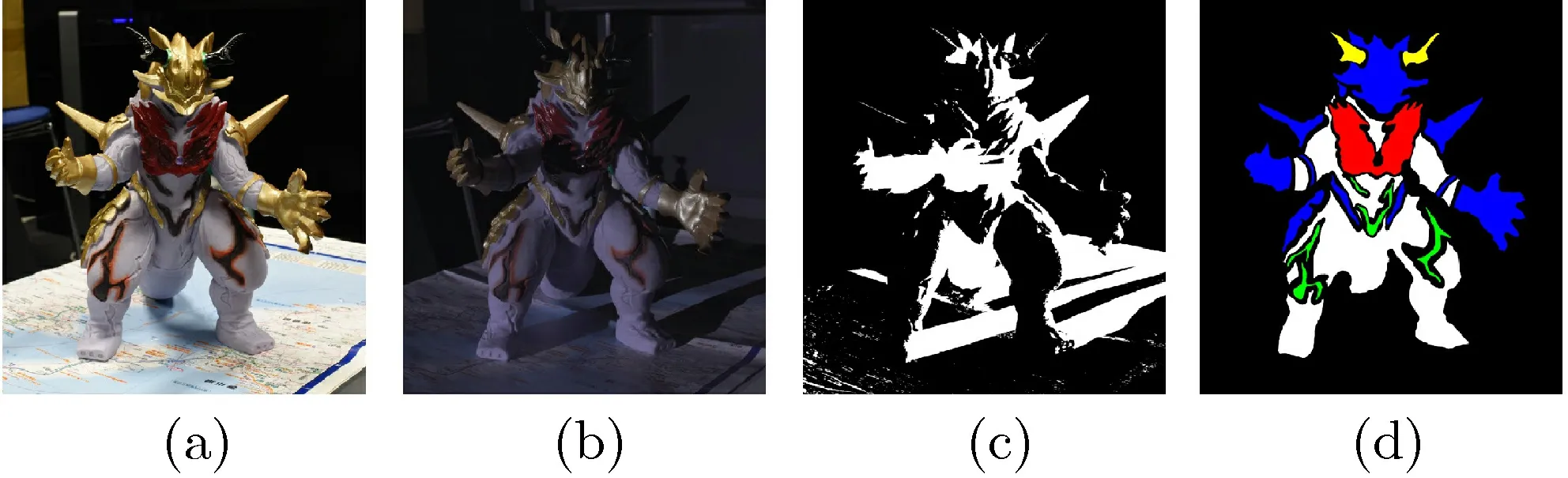
Fig. 15 (a) One of the multi-view images for acquiring geometry. 67 images were used. (b) One of the distant light images for acquiring the reflectance distribution. Eight images were used. (c) One of the shadow mask images. Eight images were used. (d) One of the masks for material separation. Eight images were used.
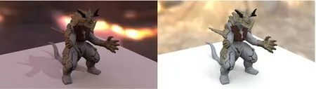
Fig. 16 Images rendered using the reconstructed BRDF with two lighting environments (Paul Debevec 1998, 1999).
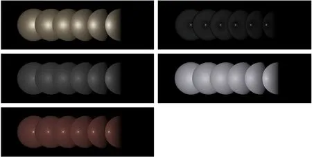
Fig. 17 Rendered sphere with BRDFs reconstructed from the gold part(upper left),black horn part(upper right),black line part(middle left), purple body part (lower left), and red chest part (lower left).
Figure 16 shows rendered results using the reconstructed BRDFs, and Fig. 17 shows spheres rendered with reconstructed BRDFs for several lighting directions. In Fig. 17, different colors and shapes of specularity are reconstructed from each part,and their appearance is very plausible, as shown in Fig. 16.
Lacquerware.Additionally, we reconstructed the BRDF of the lacquerware plate shown in Fig. 18(a).We used 105 multi-view images to acquire the geometry and captured eight distant light images for acquiring the reflectance (Fig. 18(b)). These distant light images were captured so as to contain the specular peak of every material. For this experiment,we captured distant light images several times because of the high specularity. We separated the lacquerware into three parts and manually constructed the masks for material separation (Fig. 18(c)).
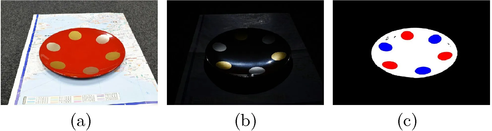
Fig. 18 (a) Example of multi-view images. (b) Example of distant light images. (c) Example of mask images.
Figure 19 shows the reconstructed result. We have smoothed the reconstructed surface for visualization.For BRDF reconstruction, we used the reconstructed geometry without smoothing. From these images, we can observe the glossy specular nature of the redcoated area and the spread specularity of the silver and gold areas. These results are very plausible when compared with the input images.
These plausible results indicate that the proposed method may be effective for digital reproduction of cultural objects, e.g., for digital archiving.
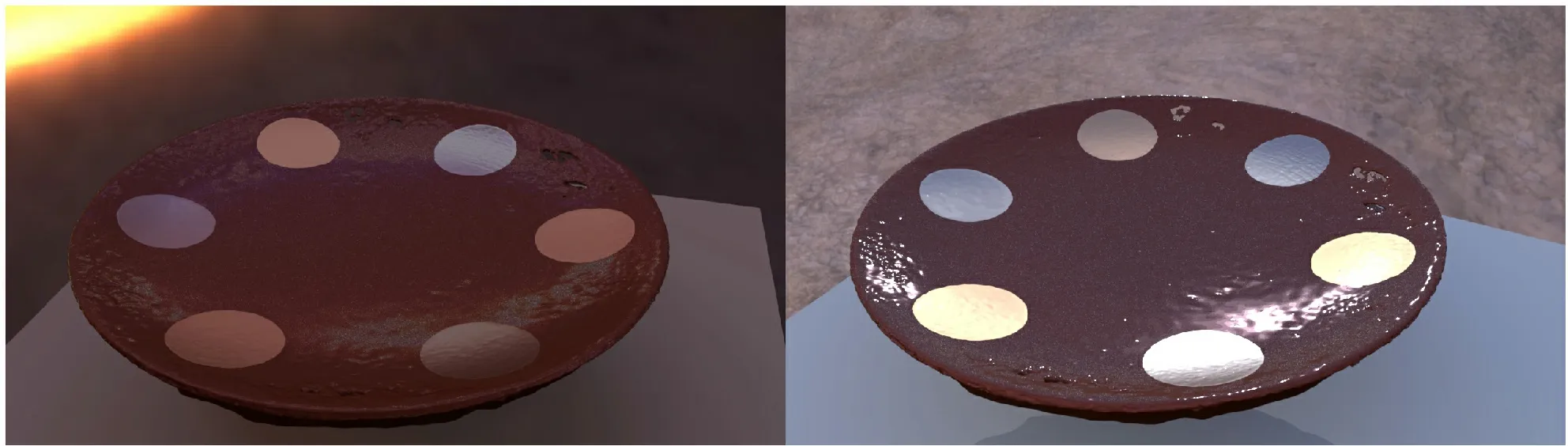
Fig. 19 Rendered images using the reconstructed BRDF with two lighting environments (Paul Debevec 1998, 1999).
6.2 Outdoors experiments
We also reconstructed the BRDF of an object located in an outdoor environment: see Fig. 20. Figure 20(a) is an example of the images used to acquire the geometry. We also acquired reflectance values from these images by assuming the Sun to be the distant light source. We determined the sunlight direction from the time and location of the pictures. We separated the pole into two areas,the central metallic area and the other parts, and excluded the areas of peeling paint. We then individually reconstructed the BRDFs for these two areas.
Figures 20(b)and 20(c)show images rendered with the reconstructed BRDFs. Even though this outdoors approach is very rough, we can observe the plausible appearance of the main part of the pole. However,the BRDF of the metallic part is implausible because the mirror-like appearance of this part is influenced by the surrounding environment.
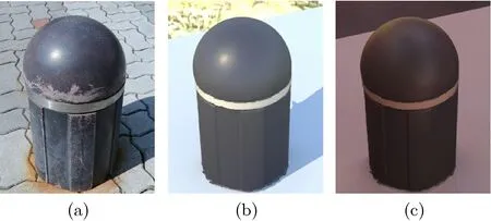
Fig. 20 (a) Example input multi-view image. (b, c) Images rendered using the reconstructed BRDFs.
Our method can work well in outdoor environments. This demonstrates the practicability of our method: MVS is often applied to outdoor objects.
7 Conclusions and future work
In this paper, we described a practical technique for BRDF reconstruction from real objects using geometry reconstructed from multi-view images. Our method requires multi-view images for geometry reconstruction and a few additional images to acquire the reflectance. The main contributions of this work are the three assumptions used to determine which regions have reliably reconstructed surface normals.Our method has high practicability because it requires only a few additional operations to the existing MVS pipeline, and there are no complex setups or special devices. The experimental results acquired by our method are plausible in both indoor and outdoor environments.
The workflow of our method is completely isolated from that of MVS. Perhaps it would be more reasonable to estimate 3D shape and BRDF simultaneously. However, in this paper, we have tackled a more difficult problem based on a blind approach to the reconstruction method. The potential advantage of our approach is the separation of the 3D reconstruction method from the BRDF reconstruction method. If the 3D reconstruction method were to be replaced by a newer and better algorithm, our BRDF reconstruction method would still be applicable.
In all experiments, we empirically determined the curvature threshold and the number of samples.In future, we will analyze which values are best for BRDF reconstruction. Currently we have only evaluated the BRDF reconstructed from six samples.We will conduct further evaluations of the accuracy of the BRDF estimated from different numbers of samples or using all samples. Additionally, we need to evaluate our method by reference and/or ground truth comparisons to real measured examples.However,it is difficult to measure ground truth BRDF data without very expensive equipment. Moreover,preparing an object for which BRDF has been measured as a reference is also difficult because the actual measured object is difficult to obtain.Furthermore, our method has been applied to only one MVS algorithm. The algorithm we used is popular, but we will examine other MVS algorithms to validate the generality of our method. These further evaluations remain important parts of our future work. Additionally, the current method can only be applied to objects composed of a few materials.In the future, it will be necessary to deal with more complicated objects made of many materials. Finally,our method can acquire plausible BRDFs, so it seems feasible to update the reconstructed surface normal using the acquired BRDFs.
Acknowledgements
This work was partly supported by JSPS KAKENHI JP15K16027, JP26700013, JP15H05918, JP19H04138,JST CREST JP179423, and the Foundation for Nara Institute of Science and Technology.
Open AccessThis article is licensed under a Creative Commons Attribution 4.0 International License, which permits use, sharing, adaptation, distribution and reproduction in any medium or format,as long as you give appropriate credit to the original author(s)and the source, provide a link to the Creative Commons licence, and indicate if changes were made.
The images or other third party material in this article are included in the article’s Creative Commons licence, unless indicated otherwise in a credit line to the material. If material is not included in the article’s Creative Commons licence and your intended use is not permitted by statutory regulation or exceeds the permitted use,you will need to obtain permission directly from the copyright holder.
To view a copy of this licence, visit http://creativecommons.org/licenses/by/4.0/.
Other papers from this open access journal are available free of charge from http://www.springer.com/journal/41095.To submit a manuscript, please go to https://www.editorialmanager.com/cvmj.
杂志排行

Computational Visual Media的其它文章
- Reconstructing piecewise planar scenes with multi-view regularization
- Evaluation of modified adaptive k-means segmentation algorithm
- Mixed reality based respiratory liver tumor puncture navigation
- InSocialNet: Interactive visual analytics for role–event videos
- Adaptive deep residual network for single image super-resolution
- A three-stage real-time detector for traffic signs in large panoramas