Single image shadow removal by optimization using non-shadow anchor values

Saritha Murali(),V.K.Govindan,and Saidalavi Kalady

Abstract Shadow removal has evolved as a preprocessing step for various computer vision tasks.Several studies have been carried out over the past two decades to eliminate shadows from videos and images.Accurate shadow detection is an open problem because it is often considered difficult to interpret whether the darkness of a surface is contributed by a shadow incident on it or not.This paper introduces a color-model based technique to remove shadows from images. We formulate shadow removal as an optimization problem that minimizes the dissimilarities between a shadow area and its non-shadow counterpart.To achieve this,we map each shadow region to a set of non-shadow pixels,and compute an anchor value from the non-shadow pixels.The shadow region is then modi fi ed using a factor computed from the anchor value using particle swarm optimization.We demonstrate the efficiency of our technique on indoor shadows,outdoor shadows,soft shadows,and document shadows,both qualitatively and quantitatively.

Keywordsmean-shift segmentation;particle swarm optimization; HSV;YCbCr; anchor values

1 Introduction

1Department of Computer Science and Engineering,National Institute of Technology Calicut,Kerala 673601,India.E-mail:S.Murali,saritha.mkv@gmail.com();V.K.Govindan,vkg@nitc.ac.in;S.Kalady,said@nitc.ac.in.

Manuscript received:2019-01-29;accepted:2019-05-18 geometry of the obstructing object,and the distance between the object and the surface.For instance,at different time of day,the shadow cast by the Sun on the ground changes dramatically depending on the elevation angle between the Sun and the horizon.Shadows are shorter at noon when the elevation angle is large,and are larger early or late in the day when the elevation angle is small.

The presence of shadows in images and videos reduces the success rate of machine vision applications such as edge extraction,object identi fi cation,object counting,and image matching. Some scenarios in which shadowsaffectdifferentapplications are demonstrated in Fig.1.Image segmentation techniques may incorrectly classify a shadow region as an object or as a portion of an object.This misclassi fi cation may in turn affect the detection of objects,as shown in Fig.1(a)where the part of the pavement in shadow is misclassi fi ed as a portion of the brick seat.Shadows may also cause object merging in video tracking systems. Figure 1(b)illustrates a case in which two vehicles are merged and counted as a single object due to the connecting shadow region.Shadows can also obstruct image interpretation in remote-sensing images,and thus prevent target detection(e.g.,locating roads),as demonstrated in Fig.1(c).The challenge posed by illumination inconsistencies,especially shadows,in the lane detection module of driver assistance systems is mentioned in Ref.[1].

Based on their density(i.e.,darkness),shadows can be classi fi ed into hard shadows and soft shadows.As the name indicates,hard shadows have high density,and the surface texture is nearly destroyed.On the other hand,soft shadows have low density,and their boundaries are usually diffused to the non-shadow surroundings.Furthermore,the shadow generated by obstruction of a non-point light source by an object has two distinct regions,the umbra and penumbra.The umbra is the high density region,lying towards the inner shadow area,while the penumbra is the low density region,lying towards the outer shadow area.Each of these shadow areas is depicted in Fig.2.

Fig.1 Shadows causing problems in(a)object detection,(b)traffic monitoring,and(c)interpretation of remote-sensing images.

Over the past two decades,numerous studies have been conducted on the detection and removal of shadows appearing in images[2,3]and videos[4].Shadow elimination from a single image is more challenging since the only source of information available is that single image,and there is no context.Removal of shadows is often considered to be a relighting task in which the brightness of shadow pixels is increased to make them as well illuminated as the non-shadow surroundings.In the survey[5],shadow removal techniques are categorized into reintegration methods[6],relighting methods[7],patch-based methods[8],and color transfer methods[9]. Furthermore,these techniques are either automatic[7]or interactive[10],depending on whether the user is provided an interface to incorporate his knowledge into the system.Various works related to shadow removal are presented in the next section.

The rest of this paper is structured as follows.A concise view of the state-of-the-art shadow removal techniques is presented in Section 2.Section 3 brie fl y discusses background information related to the proposed work.Section 4 details our proposed shadow elimination framework.Experimental results and comparison with other shadow removal algorithms are included in Section 5. Section 6 discusses applications and limitations of the proposed method,and Section 7 concludes the paper with some observations on possible future enhancements to the proposed method.

2 Previous work

Fig.2 Types of shadow:(a)hard shadow,(b)soft shadow,(c)shadow regions,umbra and penumbra.

Several methods are available for shadow elimination from indoor images,natural images,satellite images,and videos.Early works on shadow removal from an image are based on the assumption that camera calibration is necessary to generate a shadow-free representation,called an invariant image.Finlayson et al.[6]introduced a method to develop a shadow invariant by projecting the 2D chromaticity perpendicular to the illumination-varying direction.Another way to construct the invariant image is by minimizing entropy[11],which does not need calibrated cameras.Shadow edges are determined using edge detection on both original and invariant images.Image gradient along the shadow edges is then replaced by zeroes,followed by integration to generate the shadow-free image.These techniques require high-quality input images;however.Yang et al.[12]derived a 3D illumination invariant image from a 2D illumination invariant image and joint bilateral fi ltering.The detail layer from this 3D illumination invariant image is then transferred to the input shadow image to obtain the shadow-free image.

Baba et al.[13]used brightness information to segment an image into lit,umbra,and penumbra regions.Shadow regions are modi fi ed by adjusting the brightness and color.This method applies only to images of single textures.Features that differentiate shadow regions from their non-shadow counterparts are used for shadow detection in monochromatic images by Zhu et al.[14]. A classi fi er trained using features such as intensity,local maximum,smoothness,skewness,gradient and texture measures,entropy,and edge response is used for shadow identi fi cation.In Ref.[15],monochromatic shadows are corrected in the gradient domain by fi tting a Gaussian function for each vertical and horizontal line segment across the shadow boundary.Arbel and Hel-Or[16]showed that shadows could be cleared by adding them to a constant value in log space.Guo et al.[7]also used a scaling constant to relight shadow pixels.They used a region-based technique to detect shadows in natural images. A singleregion classi fi er and a pairwise classi fi er are trained using support vector machines(SVMs).An energy function combining these classi fi er predictions is then minimized using graph cut.Such region-based shadow removal is shown to provide better results than pixelbased methods.In Ref.[8],the best matching shadow matte is estimated for each shadow patch using a Markov random fi eld.This matte is separated from the image,leading to a shadow-free output.The technique proposed by Sasi and Govindan[17]splits and merges adjacent homogeneous quadtree blocks in the image based on a fuzzy predicate built using entropy,edge response,standard deviation,and mean of quadtree blocks.

Interactive shadow detection techniques allow users to incorporate their knowledge into the detection task.The inputs may be a quad map[9],or rough strokes[18].The work proposed by Gong and Cosker[10]requires rough scribbles in the shadow and non-shadow regions.They unwrap the penumbra boundary and perform multi-scale smoothing to derive shadow scales.A recent method by Yu et al.[19]requires the user to provide strokes on the shadow and non-shadow regions.The shadow scales are estimated using statistics of shadow-free regions,followed by illumination optimization. Certain techniques use color models which can separate illumination and re fl ectance components of the image,such as normalized RGB,c1c2c3,CIEL∗a∗b∗,and HSV to detect shadows[20].Detection using these methods mostly leads to false labeling since a pixel is classi fi ed as shadow or non-shadow without considering the neighbors.

Vicente et al.[21]mapped each shadow region to the corresponding lit region using a trained probabilistic SVM classi fi er.Each shadow region is then enhanced by matching the histogram of the shadow region with the lit region.Recent techniques for shadow detection use deep learning to learn shadow features automatically. Khan et al.[22]used deep learning for local and across-boundary features using two convolutional deep neural networks(CNNs).The most signi fi cant structural features of shadow boundaries are learned using a CNN in Ref.[23].Although the accuracy of shadow detection using feature learning is better than for non-learning approaches,the time and memory requirements for training the classi fi er are usually high. Shadow removal results may show more noise in recovered areas than surrounding non-shadow areas.In such cases,noise removal[24]is introduced as a postprocessing step to provide a seamless transition between shadow and lit areas.

This paper presents a simple,color-model based technique to remove shadows from an image.Shadow removal is modeled as an optimization task.Every pixel in a shadow segment is modi fi ed based on an anchor value computed from a set of non-shadow pixels mapped to the segment.In this way,each shadow segment is processed to acquire the fi nal shadow-free image.The method is suitable for both hard shadows and soft shadows.Also,it recovers the umbra and penumbra regions by fi nding different scale factors for these regions,and there is no need for a separate method to classify shadow pixels to umbra pixels or penumbra pixels.

The next section brie fl y introduces the color spaces used in the proposed method,the meanshift segmentation algorithm,and the particle swarm optimization(PSO)technique.

3 Background

3.1 Color spaces

Shadow regions are usually darker than their surroundings.Therefore,the creation of shadows is often attributed to the change in illumination.In RGB color space,a pixel is represented using its intensity in three different color channels,red,green,and blue,whereas in YCbCr color space,a pixel is represented in terms of its brightness and two color-difference values.To extract the illumination information from the color information,we transform the RGB image into YCbCr color space.The Y channel in YCbCr is the illumination,Cb is the blue difference,and Cr is the red difference.

In order to map shadow regions to non-shadow regions,we use HSV(hue,saturation,and value)color space.For any pixel,hue represents the basic color of the pixel,saturation represents the grayness,and value represents the brightness.Since hue is unaffected by changes in illumination,we assume that shadows,which are caused by changes in illumination,do not alter the hues of pixels.

3.2 Mean-shift segmentation

Our shadow removal system requires the input shadow image to be segmented into constituent regions.For this purpose,we use a non-parametric clustering technique called mean-shift clustering,introduced by Fukunaga and Hostetler[25].In this,we cluster pixels in RGB space.Pixels with similar colors in RGB color space are gathered into the same cluster.Pixels are recolored according to their cluster,resulting in the segmented image.

The mean-shift method models feature points using a probability density function where local maxima or modes correspond to dense areas.Gradient ascent is performed on the estimated density of each data point until the algorithm converges.All data points belonging to a particular stationary point are grouped into a single cluster.The mean-shift algorithm can be summarized as follows:

·For each sampleti, fi nd the mean-shift vectorM(ti).

·Shift the density estimation window fromtitoti+M(ti).

·Repeat until the samples reach equilibrium(i.e.,convergence).

We use the Edge Detection and Image SegmentationSystem (EDISON)developedin the Robust Image Understanding Laboratory at Rutgers University[26-28]to perform mean-shift segmentation.

3.3 Particle swarm optimization

In our work,the removal of shadows is achieved by solving an optimization problem.The objective of this optimization problem is to maximize the similarity between a shadow area and its non-shadow counterpart.It is solved using particle swarm optimization(PSO)[29].PSO was developed to model the social behavior of an animal in its group,for instance,the movement of each bird within a fl ock.The algorithm starts with a group of possible solutions called particles and moves these particles in the space based on their velocity and position.The position of a particle depends on the best position of the individual particle,and of the group.This is repeated until a solution is obtained.

4 Shadow removal by optimization

The central objective of shadow removal techniques is to achieve a seamless transition between the shadow and its surroundings by reducing the difference in intensities of the shadow area and its surroundings.Our novel approach to removing shadows by minimizing this difference is detailed in this section.Figure 3 depicts the work fl ow of the proposed method for shadow removal.The input to our system is a color image containing shadowed as well as non-shadowed areas. Shadow regions are detected using the method in Ref.[7].Image segmentation is done using mean-shift segmentation[27],and each segment is given a unique segment identi fi er(SID).

Our shadow removal algorithm is divided into four stages:(i)decomposition of the image into frameworks,(ii)initial shadow enhancement,(iii)shadow to non-shadow mapping,and(iv)shadow correction.Each of these steps is detailed in the subsections that follow.

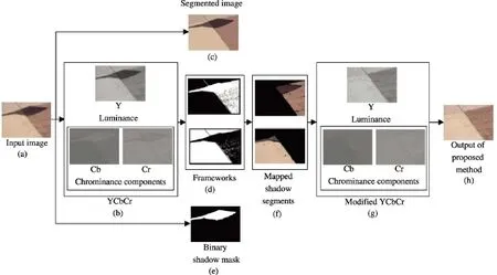
Fig.3 Overall work fl ow of our proposed shadow removal framework:(a)input shadow image,(b)input image in YCbCr space,(c)mean-shift segmentation of input image,(d)image decomposed into frameworks,(e)binary shadow mask with shadow regions in white,(f)shadow segments mapped to non-shadow regions,(g)YCbCr image after shadow removal,and(h) fi nal shadow-free output in RGB space.

4.1 Splitting the image into frameworks

Barrow and Tenenbaum[30]proposed that the formation of any Lambertian image(I)can be modeled using:

Iis the Hadamard product(°)of the re fl ectance component(R)and the illumination component(L).Since shadows occur in less illuminated areas,we segment the image into different frameworks based on the pixel illumination,so that each framework contains pixels with similar illumination. For instance,pixels belonging to hard shadow on a surface would constitute a framework.The concept of splitting the image into frameworks is adopted from the tone-mapping method for high dynamic range(HDR)images proposed in Ref.[31].

Initially,thelog10of the input image illumination is clustered using thek-means algorithm.For this purpose,the centroids are initialized to values starting from the lowest to the highest illumination of the intensity image with a step size of ten units.The fi nal set of centroids obtained after convergence of the algorithm represents the frameworks.These frameworks are further re fi ned by discarding the centroids with zero pixel membership.To restrict distinct frameworks with very close illumination,centroid pairs with a difference of less than 0.05 are iteratively merged.IfCiandCi+1are two adjacent centroids to be merged,withNiandNi+1pixels in each respectively,the new centroid valueCjon mergingCiandCi+1is given by

For a pixel at positioni,the probability of its membership of each framework is computed as the Gaussian of the difference of pixel illumination(Yi)and the centroid representing the framework(Cj).A pixel is classi fi ed into the framework for which its probability is maximum.LetFidenote the framework to which theithpixel belongs.Then the probability of theithpixel belonging to thejthframework is given by

whereσdenotes the maximum distance between any two adjacent centroids.Frameworks that contain no pixels with a probability greater than 0.3 are removed by combining them with adjacent frameworks.Finally,the framework to which each pixel belongs is recomputed as mentioned above.

4.2 Initial shadow correction

An initial enhancement of the shadow regions is performed as a pre-processing step to aid the shadow to non-shadow mapping done in the next phase of our algorithm.In this step,the shadow regions are roughly enhanced to make them better match the nonshadow equivalents.At fi rst,unwanted texture details are removed by applying a mean fi lter of window size 11×11 to the input shadow image.Further,each shadow pixel is enhanced by using a factor computed from the pixels constituting the dominant framework(the one with the most pixels).LetPindicate the pixels belonging to this framework,and¯RP,¯GP,and¯BPindicate the mean values of these pixels in each color plane in the fi ltered imageZ.LetXdenote the color plane for which the mean value is the lowest.Then the factorfis computed as

Shadow pixels are then modi fi ed using:

The output image from this stage is used for mapping shadow regions to corresponding nonshadow regions in the next step.

4.3 Shadow to non-shadow mapping

The objective of this step is to fi nd the matching set of non-shadow pixels for each shadow segment.An image can contain several disconnected shadow regions,and a single shadow region can contain multiple segments in the segmentation result.LetSIDSandSIDNindicate the segment IDs of all shadow pixels,and the segment IDs of all non-shadow pixels,respectively. Each shadow segment(unique(SIDS))is processed separately in our method.For this purpose,the image obtained from the initial shadow correction in the previous stage is converted into HSV color space.The shadow segments are mapped to a set of non-shadow pixels based on hue-matching.The hue-matching procedure is described in Algorithm 1.

4.4 Shadow removal

Once the shadow to non-shadow mappings are available,shadow removal is done by modifying the Y,Cb,and Cr planes of the input image.For each mapping,we select the framework to which the most non-shadow pixels in this mapping belongs.All non-shadow pixels in this framework are selected as candidate pixels.This is followed by computation of an anchor value(A)from the candidate pixels by selecting the highest intensity value after discardingthe top 5%intensities in each plane[32].In this way,separate anchor values are computed for the Y,Cb,and Cr planes.These anchor values are the nonshadow intensities to which the shadow intensities can be related.The shadow pixels in each segment are modi fi ed in the Y,Cb,and Cr planes as follows:

Algorithm 1 Hue-matching for shadow to non-shadow mapping

where s and c indicate the shadow segment and the mapped set of candidate pixels,respectively.The threshold of 0.4 for Eq.(10)was computed by including all images present in the dataset given by Guo et al.[7].These constraints ensure that shadow segments are modi fi ed such that their mean values become closer to those of the non-shadow regions.At this stage,certain pixels,particularly those near the shadow boundary,may be over-corrected.To address this issue,the shadow pixels for which the modi fi ed value exceeds the anchor value in the illumination plane are considered as a separate segment and are processed separately.The modi fi ed image in log space is fi nally converted into intensity space,and then to RGB.

5 Experimental results

This section present results of our shadow removal technique and a comparison with some of the available methods for shadow removal from images.Implementation ofthealgorithm and allthe experimentation was done in MATLAB R2017a on an Intel Core i5-4570 CPU@3.20 GHz with 8 GB RAM.For evaluation,the 76 images from the UIUC dataset[7]were divided into two classes based on the method used by the authors to generate the shadowless ground truth images.Set A consists of 46 images for which the ground truth is created by removing the object causing shadow.Set B consists of 30 images for which the ground truth is captured by removing the light source responsible for the appearance of shadow.We also evaluated the performance of the proposed shadow removal method on images from the ISTD[33]and LRSS datasets[8].

5.1 Qualitative analysis

To illustrate the visual quality of the output of the proposed method,various examples are included in Fig.4 and Fig.5.The fi gures also include the outputs obtained using other shadow removal methods.In Fig.4,the results displayed are for fi ve images from the UIUC dataset;the fi rst three images are from Set A,and the next two images are from Set B.For each example,the input shadow image and the corresponding shadow-free ground truth are included in rows(a)and(i),respectively.The shadow region of the input image in Fig.4(i)(a)has two different segments-one with a yellow background,and the other with a gray background.Most existing methods fail to handle the individual shadow segments,which is clear from the images in Figs.4(i)(c-f). Our proposed method handles each shadow segment separately,and the result is better than those of other methods.Figure 4(ii)also illustrates a similar case.Guo et al.[7]and Yu et al.[19]were unable to handle the shadow on the yellow lines.Zhang et al.[34]and Gryka et al.[8]failed to remove the shadow.The outputs obtained by Su and Chen[35]and Gong and Cosker[10]have artifacts near the lower region of the shadow.

Although the results in Fig.4(iii)appear to be good for most of the methods,several visual artifacts can be seen on close observation.Figure 4(iv)(b)demonstrates the scenario in which dark regions in an object are misclassi fi ed as shadows by Guo et al.[7],resulting in undesirable modi fi cation of these non-shadow regions.Gryka et al.[8]was unable to present a visually pleasing result for the same image.Even though the shadow appears to be removed in the image in Fig.4(v)(b),the text on the box is lost.Also,the attempt to remove shadows using Ref.[34]results in the false coloring of the shadow region,as shown in Fig.4(v)(d).The shadow-removal results of the state-of-the-art methods and the proposed method for the 76 images in the UIUC dataset are included in the Electronic Supplementary Material(ESM).

Figure 5 compares the shadow removal results of various methods on 450 images from the ISTD dataset.Row(a)shows the input shadow images,while row(f)shows the corresponding shadow-free ground truths.Figure 5(i)illustrates the efficiency of the proposed method in removing hard shadows.The image in Fig.5(ii)(a)has a dark region which is misclassi fi ed as shadow region by the methods in rows(b-d).The soft shadow in Fig.5(v)(a)is efficiently removed by our method.For all the input shadow images,our proposed method gives better results than other stateof-the-art shadow removal techniques.

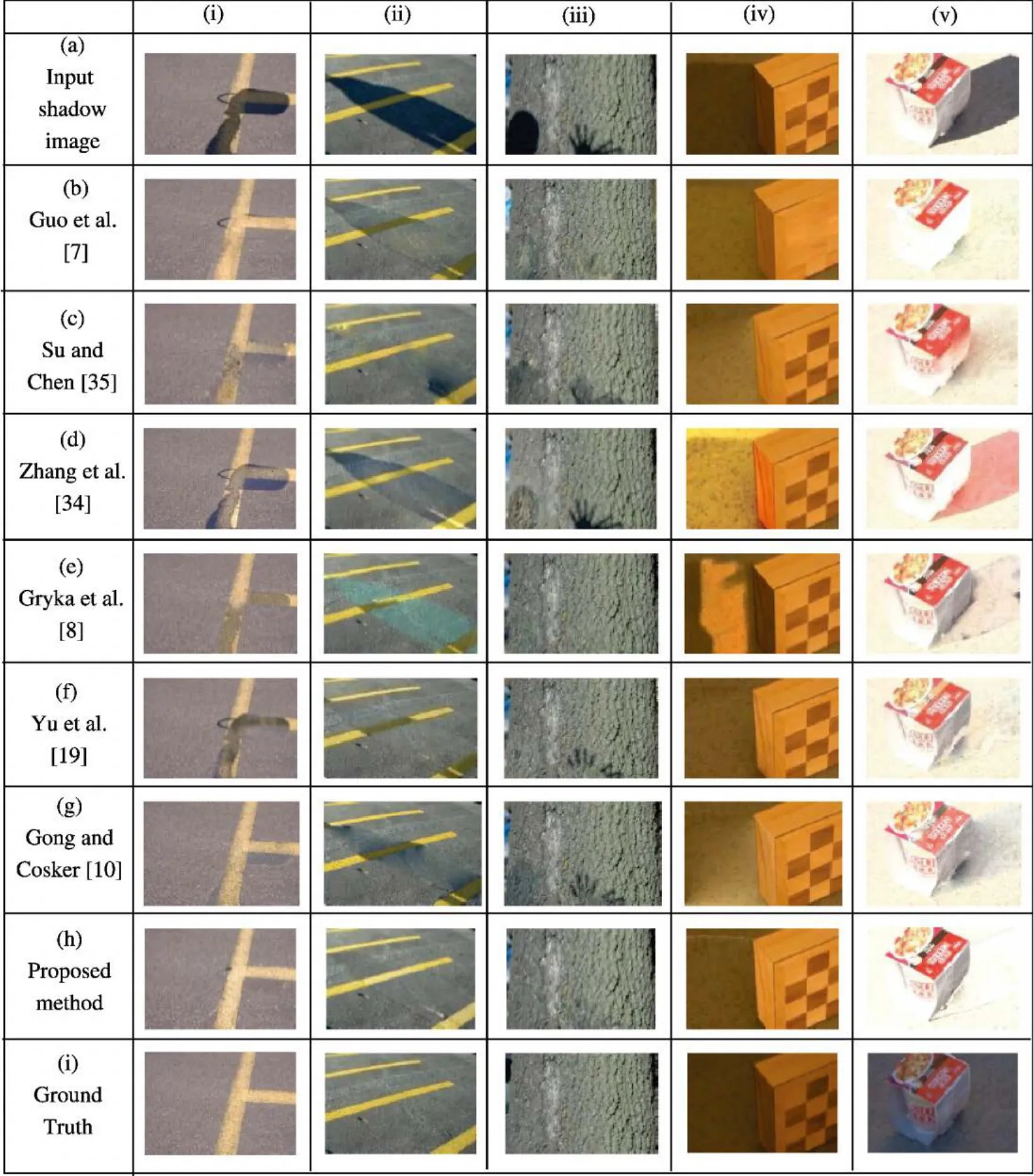
Fig.4 Comparison of shadow removal techniques using images from the UIUC dataset.Row(a)shows the original shadow images.Row(i)shows the corresponding shadow-free ground truths.Rows(b-h)contain results using the approach named in the fi rst column.

5.2 Quantitative analysis

This section analyzes the accuracy of the proposed method in removing shadows from images using the three different metrics described below.

5.2.1Root mean-squared error(RMSE)

RMSE is the square root of the mean of the squared error.The error for an image is computed as the per-pixel difference between the shadow-free ground truth and the shadow removal output.LetGiandOiindicate the intensity of theithpixel in the ground truth and the output images,respectively.Then the RMSE of ann-pixel image is computed by Since RMSE is an error measure,a lower value indicates that the output image is more similar to the ground truth.

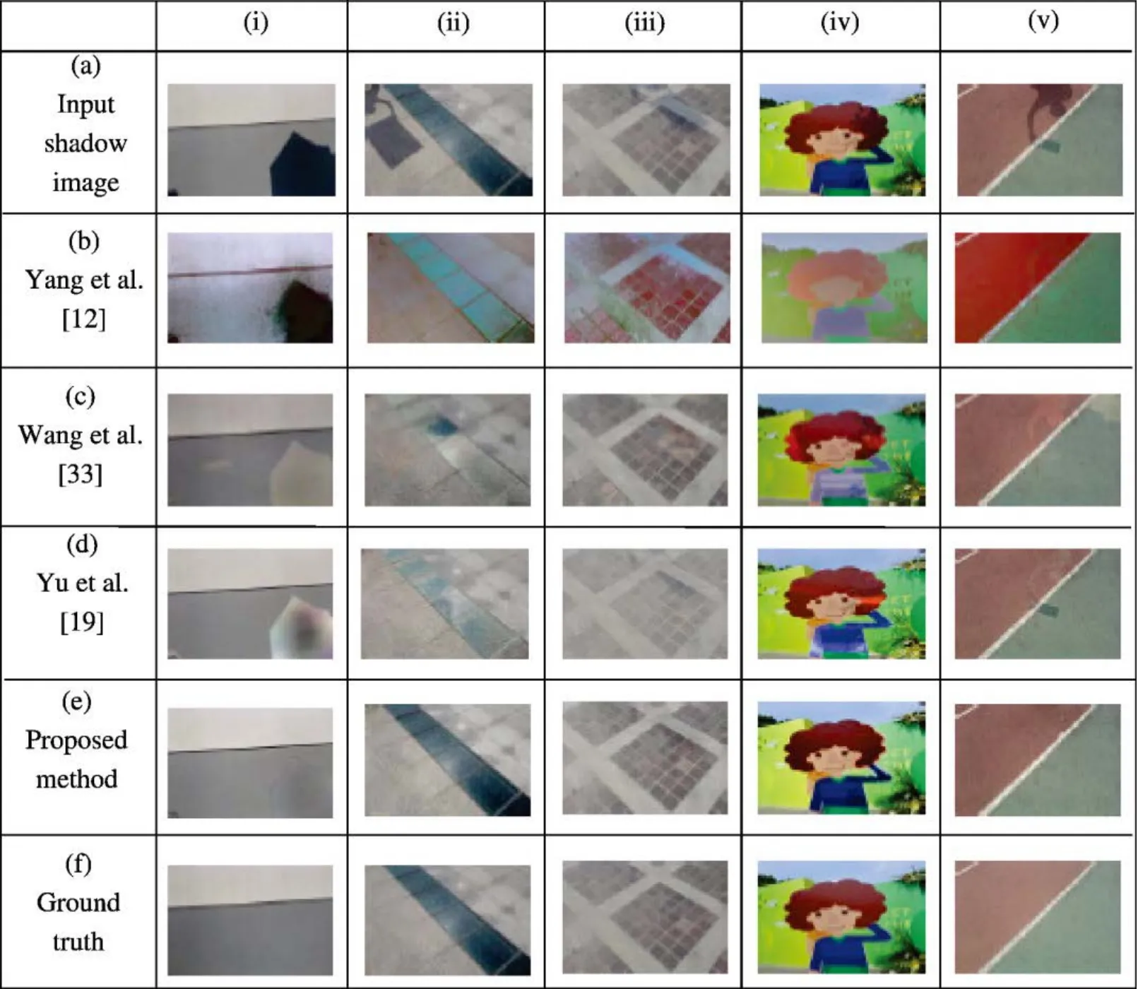
Fig.5 Comparison of shadow removal techniques using images from the ISTD dataset.Row(a)has the original shadow images.Row(f)has the corresponding shadow-free ground truths.Rows(b-e)contain results using the approach named in the fi rst column.

5.2.2Peak signal to noise ratio(PSNR)

PSNR is used to fi nd peak error.It computes the peak value of SNR,in decibels,between two images.The value of PSNR ranges between 0 and in fi nity.A higher PSNR value signi fi es better quality of the output image.Initially,we compute the mean-squared error(MSE)between the shadow-free ground truth and the shadow removal output as below:

whereGiandOiindicate the intensity of theithpixel in the ground truth and output images,respectively.Then the PSNR is computed using:

whereηdenotes the maximum possible pixel value in the images.

5.2.3Structural similarity index(SSIM)

SSIM is a metric used to compute the correlation between two images.It is considered to be a measure that is closest to the human visual system.The SSIM formula given in Eq.(14)is a weighted combination of comparisons of three elements between the images,namely luminance,contrast,and structure:

whereGandOare the shadow-free ground truth and the shadow removal output,respectively,µGandµOare the mean values ofGandO,σ2Gandσ2Oare the variances ofGandO,andσGOis the covariance ofGandO.c1andc2are variables computed using the dynamic range of pixels.

The average values of RMSE,PSNR,and SSIM for the two sets of images in the UIUC dataset are tabulated in Table 1.We have computed separate RMSE for shadow areas,non-shadow areas,and the entire image.The average values of RMSE,PSNR,and SSIM of the original shadow image with the corresponding ground truths are included in the fi rst row of each table.Imperfect shadow detection has resulted in non-zero RMSE in the nonshadow regions of the original shadow images and the corresponding ground truths.Another reason for this is the misalignment of the input images and the ground truths.Variations may also arise due to changes in the direct and ambient light reaching the non-shadow surface on removal of the shadow source.The values in Table 1 indicate that our results are superior to those of other methods.

The reason for partitioning the images in the UIUC dataset into Set A and Set B can be explained by comparing the fi rst rows in Table 1(a)and Table 1(b).The shadow-free ground truths for Set B images are darker than their corresponding shadow images since these ground truths are generated by eliminating the light sources causing the shadow(e.g.,see Fig.4(v)).Hence,the shadow region of the ground truth is more similar to the shadow region of the original image than the results of various shadow removal techniques.This explains the lower shadow region RMSE,and the higher non-shadow region RMSE of images in Set B for the original shadow images.This reason also explains the higher PSNR and SSIM values.

Quantitative results on 450 images from the ISTD dataset[33]are included in Table 2.The values in the table indicate that the proposed method performs better than other state-of-the-art shadow removal techniques.

Also,to analyze the effectiveness of our shadow removal approach,we conducted experiments on images with soft shadows.A method to remove soft shadows from images was proposed in Ref.[8].A quantitative analysis done on 15 images from their dataset is included in Table 3.The shadow-freeground truths and the results using other methods were made available by the authors.The average values of RMSE,PSNR,and SSIM in the table indicate that the proposed method can be used to remove soft shadows from images efficiently.

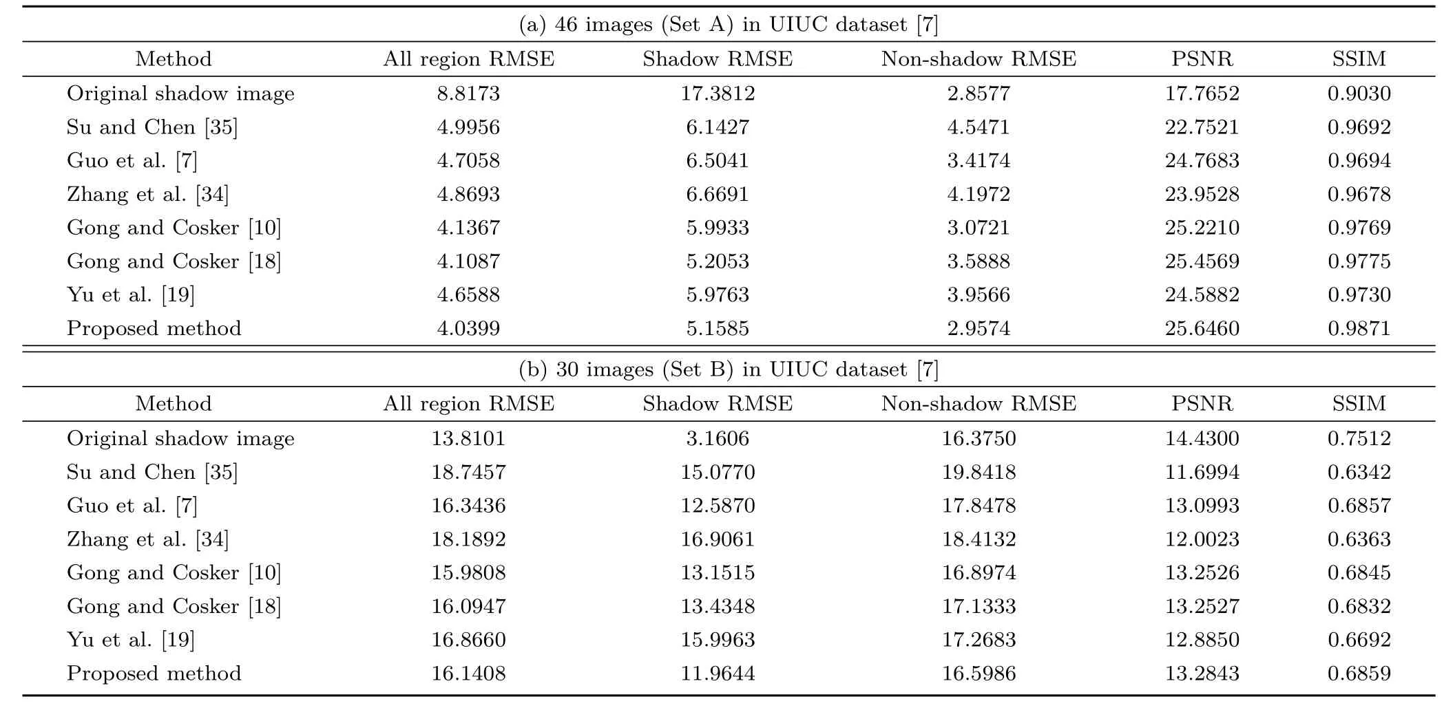
Table 1 Quantitative results on the images from the UIUC dataset[7].(a)Images for which the ground truth is created by removing the object causing shadow.(b)Images for which the ground truth is created by removing the light source responsible for the appearance of the shadow.Values are averages computed over the set of images

Table 2 Quantitative results for 450 images from the ISTD dataset[33].The values are averages computed over the set of images

Table 3 Quantitative results on 15 images from the soft shadows dataset given by Gryka et al.[8].The values are averages computed on the set of images

6 Discussion

6.1 Need for initial shadow correction

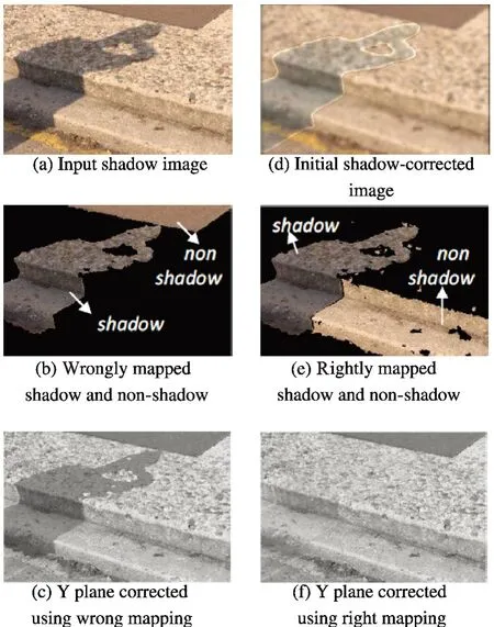
Fig.6 Need for initial shadow correction.

Figure 6 demonstrates the need for initial shadow correction as a pre-processing step to improve the accuracy of shadow to non-shadow mapping.The left column(Figs.6(a)-6(c))illustrates the case in which the input image itself is used for hue-matching to fi nd the shadow to non-shadow mapping.The second column(Figs.6(d)-6(f))uses the initial shadow corrected image for shadow to non-shadow mapping.It is evident from the fi gure that the shadow region is mapped to the wrong non-shadow region in the if rst case.This is because the hue values of shadow pixels are a closer match to those of the dark nonshadow region in the image.In the shadow corrected image,the illumination of the shadow region is roughly enhanced and hence the hue value of the shadow region is matched to the lighter non-shadow surroundings.Also,smoothing the unwanted texture details restricts the hue values in the shadow region from being distributed over a wide range of bins.

6.2 Applications

The experimental results in the previous section show the efficiency of the proposed method in removing shadows from indoor and outdoor images.Figure 7 demonstrates the capability of our shadow removal algorithm in removing shadows from document images.Oliveira et al.[36]and Bako et al.[37]developed shadow removal methods explicitly for document images,and Gong and Cosker[18]for general images.The results of the methods mentioned in the fi gure were obtained from Ref.[37].It is evident from Fig.7(e)that our proposed system can process shadows on document images,and the result is comparable with that of Bako et al.[37].

6.3 Limitations

Some limitations of the proposed shadow removal method are shown in Fig.8.The input shadow image in Fig.8(a)has an object that is completely covered by shadow.In this case,the proposed method fails to fi nd a matching non-shadow region for that object.This results in the object being mapped to the road and hence the result in Fig.8(a)(iv).

Fig.7 Shadow removal from document images.

Figure 8(b)shows an image with shadow on a complex textured surface.The segmentation of this image produces an image in which very small objects on the ground are clustered into the same segment even though their colors(hue)are different.Also,hue-matching leads to an incorrect shadow to nonshadow mapping in this case,thereby resulting in the output shown in Fig.8(b)(iv).

Detection of soft shadows with a highly diffused penumbra is a challenging task.Figure 8(c)illustrates the effect of the shadow detection and image segmentation results of the proposed method on soft shadow images with a highly diffused penumbra.The penumbra region is not properly detected leading to improper shadow correction output.

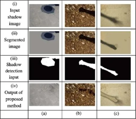
Fig.8 Failures of the proposed shadow removal method for(a)object completely in shadow,(b)shadow on a complex textured surface,and(c)soft shadow with highly diffuse penumbra.

7 Conclusions

Shadows are natural phenomenon that may lead to the incorrect execution of certain tasks in computer vision,such as object detection and counting.We have presented a simple,color-model based method to remove shadows from an image.Shadow regions are initially mapped to corresponding non-shadow regions using hue-matching.This is followed by removal of shadows using a scale factor computed using particle swarm optimization and an anchor value from the non-shadow region.This method does not require prior training,and works on both hard shadows and soft shadows.Moreover,it recovers the umbra and penumbra regions by fi nding separate scaling factors for these regions.The umbra and penumbra regions are handled separately,without requiring a classi fi er to distinguish them.Furthermore,unlike many other existing methods,our method does not alter pixels in non-shadow areas.

Our method was evaluated on various datasets,and the results quantitatively analyzed.Also,the subjective quality of the output images was illustrated using selected examples.The method works for both indoor and outdoor images,and for images under various lighting conditions.This method does not require high-quality inputs or accurate image segmentation.However,the time taken to process an image grows with the number of segments and the time needed for the PSO to converge.Also,the shadow to non-shadow mapping may lead to incorrect results if a non-shadow equivalent of a shadow segment does not exist.

Electronic Supplementary MaterialSupplementary material is available in the online version of this article at https://doi.org/10.1007/s41095-019-0148-x.

Open AccessThis article is licensed under a Creative Commons Attribution 4.0 International License,which permits use,sharing,adaptation,distribution and reproduction in any medium or format,as long as you give appropriate credit to the original author(s)and the source,provide a link to the Creative Commons licence,and indicate if changes were made.

The images or other third party material in this article are included in the article’s Creative Commons licence,unless indicated otherwise in a credit line to the material.If material is not included in the article’s Creative Commons licence and your intended use is not permitted by statutory regulation or exceeds the permitted use,you will need to obtain permission directly from the copyright holder.

To view a copy ofthis licence, visit http://creativecommons.org/licenses/by/4.0/.

Other papers from this open access journal are available free of charge from http://www.springer.com/journal/41095.To submit a manuscript,please go to https://www.editorialmanager.com/cvmj.