ASYMPTOTIC NORMALITY OF THE NONPARAMETRIC KERNEL ESTIMATION OF THE CONDITIONAL HAZARD FUNCTION FOR LEFT-TRUNCATED AND DEPENDENT DATA∗†

Meijuan Ou,Xianzhu Xiong,Yi Wang

(College of Math.and Computer Science,Fuzhou University,Fuzhou 350116,Fujian,PR China)

Abstract Under some mild conditions,we derive the asymptotic normality of the Nadaraya-Watson and local linear estimators of the conditional hazard function for left-truncated and dependent data.The estimators were proposed by Liang and Ould-Saïd[1].The results confirm the guess in Liang and Ould-Saïd[1].

Keywords asymptotic normality;Nadaraya-Watson estimation;local linear estimation;conditional hazard function;left-truncated data

1 Introduction

Left-truncated data often occurs in astronomy,economics,epidemiology and biometry;see,e.g.,Woodroofe[2],Feigelson and Babu[3],Wang et al.[4],He and Yang[5].Since Ould-Saïd and Lemdani[6]proposed a new nonparametric estimator(of NW type)of the nonparametric regression function under a left-truncation model,the nonparametric statistical inference for left-truncated data has been received an increasing interest in the literatures.For the case of estimating the conditional mean function,see Liang et al.[7,8],Liang[9],Wang[10];for the case of estimating the conditional quantile function,see Lemdani et al.[11],Liang and de U˜na-Álvarez[12,13],Wang[14];for the case of estimating the conditional density function,see Ould-Saïd and Tatachak[15],Liang[16],Liang and Baek[17].

Recently,Liang and Ould-Saïd[1]proposed a plug-in weighted estimator of the conditional hazard rate for left-truncated and dependent data.They obtained asymptotic normality of the estimator and compared the finite sample performance with the Nadaraya-Watson(NW)and local linear(LL)estimators proposed by them,but they did not give the asymptotic normality of the NW and LL estimators.This paper will make up for this problem.

The rest of this paper is organized as follows.In Section 2,we first introduce the left-truncation model,some results,and the NW and LL estimators of the conditional hazard function in the left-truncation model.The asymptotic normality of the NW and LL estimators are stated in Section 3,while their proofs are given in Section 4.

2 Estimators

2.1 Preliminary

Let(Y,T)be random variables,where Y is the variable of interest(regarded as the lifetime in survival analysis)with a distributed function(df)eF(·),and T is the random left-truncation variable with a continuous d.f.G(·).In the random lefttruncation model,one can observe(Y,T)when Y≥T,whereas nothing is observed when Y0.Suppose that X is the associate covariate with a density function l(·),and(X,Y)is independent of T.Let f(·|x)and S(·|x)denote the conditional density function and the conditional survival function of Y given X=x,respectively.Then for all y∈R and S(y|x)>0,the corresponding conditional hazard function λ(y|x)equals

Let{(Xi,Yi,Ti),1≤i≤N}be a sequence of random vectors from(X,Y,T).As a result of left-truncation,n-the size of the actually observed sample,is random with n≤N and N being unknown.Since N is unknown and n is known(although random),the results are not stated with respect to the probability measure P(related to the N-sample)but involve the conditional probability P with respect to the actually observed n-sample.Also E and E denote the expectation operators under P and P,respectively.

In the sequel,the observed sample{(Xi,Yi,Ti),1≤i≤n}is assumed to be a stationary α-mixing sequence.Recall that a stationary process{Ui,i≥ 1}is called α-mixing or strongly mixing,if the α-mixing coefficient converges to 0 as n → ∞,wheredenotes the σ-algebra generated by{Ui,j≤ i≤k}.Many processes do fulfill the α-mixing property.The reader can see Doukhan[18]for a more complete discussion of the α-mixing property.

Following the idea of Lynden-Bell[19],the nonparametric maximum likelihood estimator of G(·)is given by

For any distribution function W,let aW=inf{y:W(y)>0}and bW=sup{y:W(y)<1}be its two endpoints.Throughout the paper,the star notation(∗)relates to any characteristic function of the actually observed data.Let F(·,·)and f(·,·)be the joint distribution and density functions of(X,Y),respectively.Since T is independent of(X,Y)and Y≥T,the conditional joint distribution of(X,Y,T)is

Taking t=+∞,the observed pair(X,Y)has the following distribution function F∗(·,·):

which yields that

2.2 NW and LL estimators

Liang and Ould-Saïd[1]proposed the NW and LL estimators of conditional hazard function for the left-truncated data.The NW estimator(y|x)is defined as

where

with

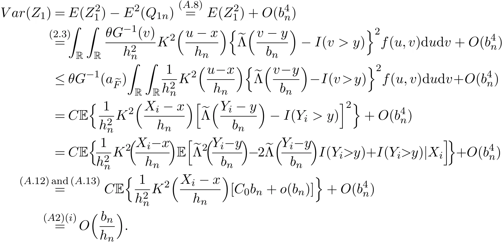
K(·)and Λ(·)are some kernel functions defined on R,Khn(·)=K(·/hn)/hn,Λbn(·)=Λ(·/bn)/bn,0

where

with

3 Assumptions and the Main Results

In the sequel,let C,C0,C1and C2denote generic finite positive constants,whose values are unimportant and may change from line to line,and U(x)represent a neighborhood of x.Set

To establish the asymptotic results,we need the following assumptions:

(A0)aG

(A1)(i)Both K(·)and Λ(·)are bounded functions with compact support on R;

(ii)∫RΛ(t)dt=1,R∫K(t)dt=1;

(iii)

RtΛ(t)dt=0,RtK(t)dt=0.

(A2)(i)The second derivatives of l(·)are bounded in U(x)and l(x)>0;

(ii)the second partial derivatives of f(·|·)are continuous in U(x) × U(y)and f(y|x)>0;

(iii)S(·|·)has continuous second partial derivatives U(x)×U(y)and S(y|x)>0;

(iv)for any y ∈ R,σ2(·,y)is continuous at x with σ2(x,y)>0.

(A3)(i)For all integers j≥1,the joint conditional density(·,·,·,·)of(X1,Xj+1,Y1,Yj+1)exists on R×R×R×R and satisfies(s1,s2,t1,t2)≤ C for(s1,s2,t1,t2)∈U(x)×U(x)×U(y)×U(y);

(ii)for all integers j≥1,the joint conditional density(·,·,·)of(X1,Xj+1,Y1)exists on R×R×R and satisfies(s1,s2,t1)≤C for(s1,s2,t1)∈U(x)×U(x)×U(y);

(iii)for all integers j≥1,the joint conditional density(·,·,·)of(X1,Xj+1,Yj+1)exists on R×R×R and satisfies(s1,s2,t2)≤C for(s1,s2,t2)∈U(x)×U(x)×U(y);

(iv)for all integers j≥1,the joint conditional density(·,·)of(X1,Xj+1)exists on R×R and satisfies(s1,s2)≤C for(s1,s2)∈U(x)×U(x).

(A4)Assume that nhnbn→∞,and for positive integers q=qnthere are qn=o((nhnbn)1/2)and

Remark 3.1 Conditions(A0),(A1)(i)(ii)(iii),(A2)(i)(ii),(A3)(i)(ii)(iii)(iv)and(A4)are the same as those of the corresponding results of Liang and Baek[17].For more detail on these conditions,we refer the reader to Remark 3.1 of Liang and Baek[17].Condition(A2)(iii)is the same as condition(A6)in Liang and Ould-Saïd[1],and condition(A2)(iii)(iv)is an adaption of condition(A5)of Liang et al.[8]by replacing ϕ(Y)with I(Y>y)here.

The main results of this paper are given as follows.

Theorem 3.1Letα(n)=O(n−λ)for someλ >3.Suppose that conditions(A0)-(A4)are satisfied.Then

whereV2(y|x)= θ∆02∇02λ(y|x)/{G(y)l(x)S(y|x)},and the asymptotic bias ofis given by

Theorem 3.2Letα(n)=O(n−λ)for someλ >3.Suppose that conditions(A0)-(A4)are satisfied.Then

where the asymptotic bias ofis given by

Remark 3.2 Note that the condition“RtK(t)dt=0”of condition(A1)(iii)b implies that∆11=0.Again by(3.2),it follows that the asymptotic bias ofλNW(y|x)is

From(3.4),it can be easily proved that the asymptotic bias ofis also(3.5),which is the same as that of.In the case that“∫RtK(t)dt≠0”,it can be proved that the asymptotic bias ofis

while the asymptotic bias ofis the same as Asb2.So we can say thathas a significative gain in the asymptotic bias term with respect toThis gain on the asymptotic bias term confirms the superiority of the local linear method over the kernel method in the context of conditional hazard estimation for left-truncated data.

Remark 3.3 It follows from Theorems 3.1,3.2 and Theorem 1 in Liang and Ould-Saïd[1]thatand the estimator(proposed by Liang and Ould-Saïd[1])have same asymptotic normality,and they have better asymptotic mean squared errors than.This is exactly what Liang and Ould-Saïd[1]guessed.

4 Proof of the Main Results

Lemma 4.1Letα(n)=O(n−λ),λ >3.Suppose that conditions(A0),(A1)(i)(ii)(iii),(A2)(i)(ii),(A3)(i)(ii)(iii)(iv)and(A4)are satisfied.Then

Remark 4.1 Lemma 4.1(2)is a direct corollary of Theorem 3.2 of Liang and Baek[17].In Liang and Baek[17],Theorem 3.1 also holds under conditions of Lemma 4.1(1)and without the condition“”,because this condition is used only in the proof of the property that ln(x)=l(x)+op(1)in Step 1,but the proof of the property that sn0=l(x)+op(1)in Step 5(note that sn0=ln(x))does not use this condition.Then Lemma 4.1(i)follows from Theorem 3.1 of Liang and Baek[17].

Lemma 4.2Letα(n)=O(n−λ),λ >3.Suppose that conditions(A0),(A1)(i)(ii)(iii),(A2)(i)(iii)(iv),(A3)(iv)and(A4)are satisfied.Then

Lemma 4.2 will be proved in Appendix A.Next we will only prove Theorem 3.1,and Theorem 3.2 can be proved similarly.

Proof of Theorem 3.1 It follows from condition(A4)that nhn→∞,which along with Lemma 4.2(1)implies that.From Lemma 4.1(1)and Slutsky,s lemma,it follows that

Note that

The asymptotic distribution of H1is given in(4.5).H2can be rewritten as

By(4.1),(4.3)and the property that

Then Theorem 3.1 follows from(4.8),(4.9)and the fact.The proof is completed.

A Appendix

Now prove Lemma 4.2.We only prove Lemma 4.2(2),and Lemma 4.2(1)can be proved similarly.

Proof of Lemma 4.2(2)By(2.9)and the property that,the sampling error ofcan be written as

First we show that

From(2.10),it follows that

From Step 5 in page 17 of Liang and Baek[17],snjl(x)∆j1,j=0,1,2.In addition,condition(A1)(ii)(iii)imply that∆01=1,∆11=0.Then(A.3)can be written as

Note that

It follows from Lemma 5.2 and the bound of J1n(x)in Step 1 of Liang and Baek[17]that

According to(A.2),(A.4),(A.5)and(A.6),(A.2)will hold if

To prove(A.7),we need to obtain

Now consider(A.8).It follows from(2.4)that

By condition(A1)and(A2)(iii),similar to the proof of Lemma A.5 in Li and Racine[20],we have

It follows from(A.10),(A.11)and condition(A2)(i)(iii)that

Then(A.8)holds.Next consider(A.9).

Set

To compute V ar(Z1).

Then

In addition,similar to the proof of J2nin Step 5 of Liang and Baek[17],we can get

Then(A.9)follows from(A.14),(A.15)and(A.16).So(A.2)holds.

Second,consider the asymptotic normality of An.From Theorem 3.2 of Liang et al.[8],by taking ϕ(Y)=I(Y>y),we have

At last,Lemma 4.2(2)follows from(A.1),(A.2)and(A.18).The proof is completed.