A recognition model of survival situations for survivable systems

Zhao Guosheng Shao Zihao Wang Jian Li Yingmei

(1College of Computer Science and Technology, Harbin Normal University, Harbin 150025, China)(2School of Computer Science and Technology, Harbin University of Science and Technology, Harbin 150080, China)

Abstract：Due to the lack of pre-recognition and post-prediction in existing survivable systems, a recognition model of survival situations for survivable systems is proposed. First, the survival situation data is clustered into several survival clusters with different service levels based on the Ward method, and then the survival clusters are classified and recognized by means of the error-eliminating decision-making method, which can realize the pre-recognition of the system’s survival situation. Secondly, the differentiated survival situation data is used to generate stationary predicting sequences. The autoregressive integrated moving average (ARIMA) model is constructed, and the stability, randomness and reversibility index of the model are verified by the auto-correlation function and partial auto-correlation function. Finally, fuzzy particles and the residual correction for the support vector regression (SVR) model are applied to realize the post-prediction of the survival situation. Compared with traditional decision-making methods, the simulation experiments show that the pre-recognition module can not only cluster the survival situation data and identify the service ranks, but can also recognize the illegal users. According to the prediction of abnormal situations numbers and residual correction, the model can effectively realize the post-prediction of survival situations for survivable systems.

Keywords：survivability; recognition; fuzzy particle; residual correction

Survivability research is a hot issue in the next generation of cyberspace security. According to the definition of Ref.[1], the research of survivability is divided into three aspects, which are resistance, recognition and recovery (3R attributes). In reality, systems are always being invaded and destroyed by different degrees, and the failures of systems are inevitable. How to use the current survival situation data to predict the future survival situations has become an urgent problem. Therefore, we focus on the pre-recognition and the post-prediction of survival situations for survivable systems.

At present, most of the existing literature focuses on the recovery and resistance research. Yaghlane et al.[2]introduced the concept of system survivability under attack in analogy with system reliability. Zhao et al.[3]described the survivability of RSCN by the fault repair and anti-failure technology in network systems. Raja et al.[4]proposed a multi-dimensional measurement method for the survivability of open source software. Most research on the recognition of survivable systems often focuses on perception. It is still in the initial stage and related literature is insufficient. Zhao et al.[5]proposed an autonomous recognition unit from the survivability of autonomous recognition. They focused on the recognition of the detection parameter definition, the autonomous recognition model and the threshold variable method. The recognition monitoring mechanism can improve the ability of self-cognition and the capacity of services, but it cannot predict future survival situations. Wang et al.[6]mainly studied the hierarchical cognitive model, the self-management model of cognitive unit and the transformation process of survival state. The proposed method improves survivability by enhancing self-recovery ability, but lacks the processing of residual data and prediction of future survival situations. Dharmaraja et al.[7]applied the concept of survivability into vehicle ad hoc network. This method created a mobile network to facilitate communication between vehicles. It can ensure the safety of roads and reduce security risks.

Therefore, existing literature on the survival situations for survivable systems can be divided into two fields. The first is the definition of survivability[2-4]. It mainly focuses on the studies of resistance and recovery. Most research belongs to pre-recognition research. The second is the application of survivability[5-7]. There is little literature in the field of recognition for survivable systems. Most research focuses on the Internet of things and artificial intelligence, such as context awareness[8], compressed sensing, etc. On the whole, there is very little literature concerning the recognition techniques, and the recognition not only includes pre-recognition of the current survival situation, but also includes the post-prediction of the future survival situation.

1 Pre-Recognition

The Ward method[9]can cluster the current situation data into survival clusters with different service levels, and then the survival clusters are classified and recognized by means of the error-eliminating decision-making method[10], which realizes the pre-recognition of the system’s survival situation.

1.1 Ward method

At the beginning of clustering, each of the situation data is regarded as a class. Two classes with the smallest sum of squares of deviations are selected for merging. In the end, all the situation data is classified as one class. Assuming thatnsituation data is divided intokclasses (G1,G2, …,Gk), the sum of the squares of data deviations and the total data deviations are

(1)

(2)

whereyiis the center of gravity;yijis thej-th data inGi; andniis the amount of data.

1.2 Error-eliminating decision-making method

In the multi-attribute decision making problem, it is assumed that the survival situation data is indicated asA={a1,a2,…,am}, and attributes areD={d1,d2,…,dn}. The decision matrix isX=(xi,j)m×n, andxi,jis the measured value. Attributes are divided into cost-type attribute and benefit-type attribute. The recognition steps are as follows:

Step1The error value of the survival situation data can be calculated byti,j(i=1,2,…,m,j∈N).

For cost-type attribute,

(3)

For benefit-type attribute,

(4)

According to Eqs.(3) and (4), the error value sequence of the dataai={ti,1,ti,2,…,ti,n}.

(5)

Step3The error loss value of the survival situation data can be calculated as

ki,j=aidji∈M′;j=1,2,…,n

(6)

Step4The error loss sequence needs to be sorted. The error loss sequenceki,1,ki,2,…,ki,ncan be seen as the pointRiin then-dimensional space. The closer to the origin, the better the data.

(7)

2 Post-Prediction

The post-prediction model based on autoregressive integrated moving average (ARIMA) is introduced[11]. The basic idea of the ARIMA model is that the data sequences formed by the predictive objects over time are regarded as a random sequence, and a certain mathematical model is used to approximate the sequence. Once the model is identified, it can predict the future value from the past and the present value of the time series.

2.1 Selection of model

In terms of usability, Kavousi-Fard et al.[12]demonstrated the feasibility of this model. Compared with the gray model[13]and the BP neural network model[14], it has the advantage of simple application, easy operation, high recognition of the result and support of mature software. This model does not require any assumed conditions and can be entered into any form of survival data time series for prediction.

2.2 Residual correction

Since the data residuals are unavoidable, the fuzzy information granularity[15]and the support vector regression (SVR) model are introduced to deal with residual data in the ARIMA model.

Fuzzy information granularity includes window division and fuzzification. For the convenience of calculation, triangular fuzzy particles are used. The formula is

(8)

wherexis the time series of the input data. For a single fuzzy particle, min, avg and max describe the minimum, average and maximum values of the survival situation data, respectively. The prediction residuals of the model are mapped to minimum, average and maximum values.

Next, the SVR machine model needs to be established. SVR is a support vector machine for regression analysis.

{(x1,y1),…,(xn,yn)} is a set of known training samples. The optimal decision function is constructed in the high-dimensional feature space. The formula is

(ωφ(xi)+b)-yi≤ε+ξi

(9)

2.3 Realization of post-prediction

Fuzzy particles are divided into three forms: low, medium and high, which are indicated by min, avg and max, respectively. The residual series data is divided into several sub sequences and classified by window. The SVR model is constructed from these input variables. These variables are formed by the previous window’s fuzzy information particle data set. The optimal decision function is constructed by predicting the fuzzy information particles and residual mean. The residual prediction value isesvr-1.

3 Simulation Experiment

3.1 Example of pre-recognition

3.1.1 Index selection

Since the recognition emphasizes the ability of a survivable system to recognize its own current survivable situation, the index system is mainly established according to the method proposed in Ref.[16]. This paper mainly considers four factors in recognition: integrity, usability, emergency and perception. The four factors can be divided into eight performance indices.

3.1.2 Data clustering

In the experiment, it is assumed that the survivable system provides five levels of service: A1 (highest), A2, A3, A4, A5 (lowest), and the performance of survival situation data is analyzed according to the above evaluation indices. The allow access level and deny access level will be defined by an expert scoring system with a discrete value, for 1 to 4, and the performance reduces gradually. Cost-type attributes include the data reuse rate and channel delay, and the rest are benefit-type attributes. The initial data is shown in Tab.1.

Tab.1 The initial data of the selected index

Tab.1 illustrates that the data multiplex rate and the channel delay may be reduced with the higher level of service, while the rest indices will be increased. At the same time, various service levels will have different survival performance indicators. The data of 250 normal users is randomly selected, among which the number of A1 level users, A2 level users, A3 level users, A4 level users and A5 level users are 15, 25, 70, 70 and 70, respectively.

By using the Ward method, the sum of the squares of deviations can be calculated by Eqs.(1) and (2). The SPSS19.0 software is used to obtain five kinds of data clustering. The clustering results generated by statistics are shown in Tab.2.

According to the clustering method and the comparison with Tab.1, it is found that the clustered service levels A1′, A2′, A3′, A4′ and A5′ are approximately equal to the clustered service levels A3, A1, A2, A5 and A4, respectively. The range of index attributes are basically consistent with the initial data classification.

3.1.3 Data recognition

We randomly selected ten groups of test data. The numbers of A1, A2, A3, A4 and A5 are 1, 1, 2, 2, 2, respectively, and two illegal users are selected. Through the calculation of situation data, the recognition results of the service level are realized in Tab.3.

Tab.2 The data clustering of service level

Tab.3 Decision matrix of test data

a1={0.025,0.003,0.007,0.016,0.007,0.021}

a2={0.245,0.146,0.124,0.181,0.061,0.114}

a3={0.259,0.138,0.126,0.173,0.056,0.117}

a4={0.084,0.068,0.093,0.121,0.042,0.083}

a5={0.211,0.145,0.098,0.184,0.047,0.089}

a6={0.131,0.077,0.064,0.079,0.035,0.086}

a8={0.199,0.128,0.105,0.147,0.035,0.107}

a9={0.036,0.002,0.064,0.021,0.019,0.028}

According to Eq.(7), the eccentric distance isR1=0.038,R2=0.382,R3=0.386,R4=0.209,R5=0.345,R6=0.205,R8=0.319, andR9=0.086. It also can be seen that the performance of eight data is sorted asa1,a9,a6,a4,a8,a5,a2, anda3. The error-eliminating decision-making method can not only recognize the error data, but also calculate the range of eccentric distances for each service level. The calculation results are shown in Tab.4, where it can be concluded thata1is A1 level users,a9is A2 level users,a6anda4are A3 level users,a8anda5are A4 level users,a2anda3are A5 level users, and others are illegal users.

Tab.4 Eccentric distance

The Ward method can be used to cluster the survival situation data into five clusters of the service level. The error-eliminating decision-making method can be used to classify the clusters of the survival data and recognize the service level of the user data. With the upgrading of the service level, the performance of the survival situation data will be improved. It means that the higher the level of service, the better the overall performance of the data.

In order to further illustrate the feasibility of this method, two traditional common decision-making methods (the ideal point method and the weighted average method) are used to sort these ten sets of data. The sorting results are shown in Tab.5.

Tab.5 Comparison of decision-making methods

From the sorting results, the traditional decision-making methods can only sort the data, while they cannot verify the ability of feasible data. In this paper, some of the erroneous data is successfully recognized by calculating the limit loss value, which not only increases the accurate processing ability and response time of the data, but also has consistent results with the traditional decision-making method.

3.2 ARIMA combinatorial model

3.2.1 ARIMA model

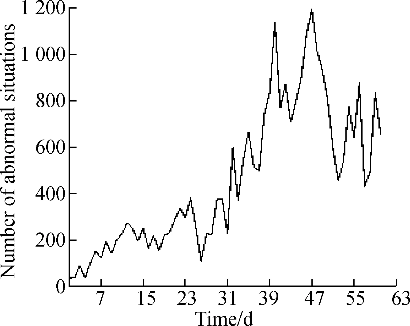
The “corrected” data in KDD99 is selected for analysis and prediction, which is used to predict the number of abnormal situations that may occur in survivable systems for the next period of time. We select 1 500 daily data, then choose the tag attribute in the last column and count the number of abnormal situations. The results are shown in Fig.1(a). The collected data sequence map illustrates that the time series data is random and non-stationary, which requires first difference processing, as shown in Fig.1(b).

(a)

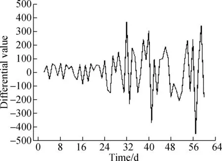
(b)Fig.1 Processing of abnormal situation with first difference.(a) Abnormal time series; (b) First difference time series

Since the difference sequence is basically distributed around 0, upper and lower sides of the scale line, it can be judged that the differential sequence is stable. The most appropriate ARIMA model is automatically generated by the use of SPSS software. The prediction results are shown in Fig.2.

In Fig.2, ARIMA (1,1,0) is the optimal prediction model. The solid line indicates the actual number of abnormal situations and the dotted line indicates the number of abnormal situations by the ARIMA (1,1,0) model. In general, the predictive results of the model are fitted with the actual situation, but accuracy is insufficient and there is a slight delay in the results.

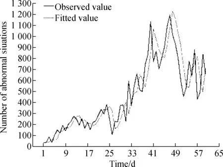
Fig.2 ARIMA (1,1,0) model prediction results

3.2.2 Information granulation and SVR model

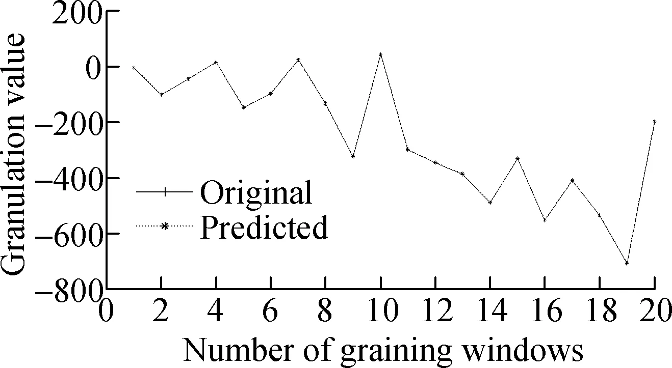
The data of 60 d is used as training sets to predict the number of abnormal situations for the next three days. Every three days’ amount of data will become a granular information window and each group of the data will blurred into three parameters (low, medium, high). This means that the sample sets for the training sets contain 20 windows and the output samples contain 21 windows, as shown in Fig.3, where low, medium and high describe the minimum, average, and maximum value of changes to the abnormal situation, respectively.

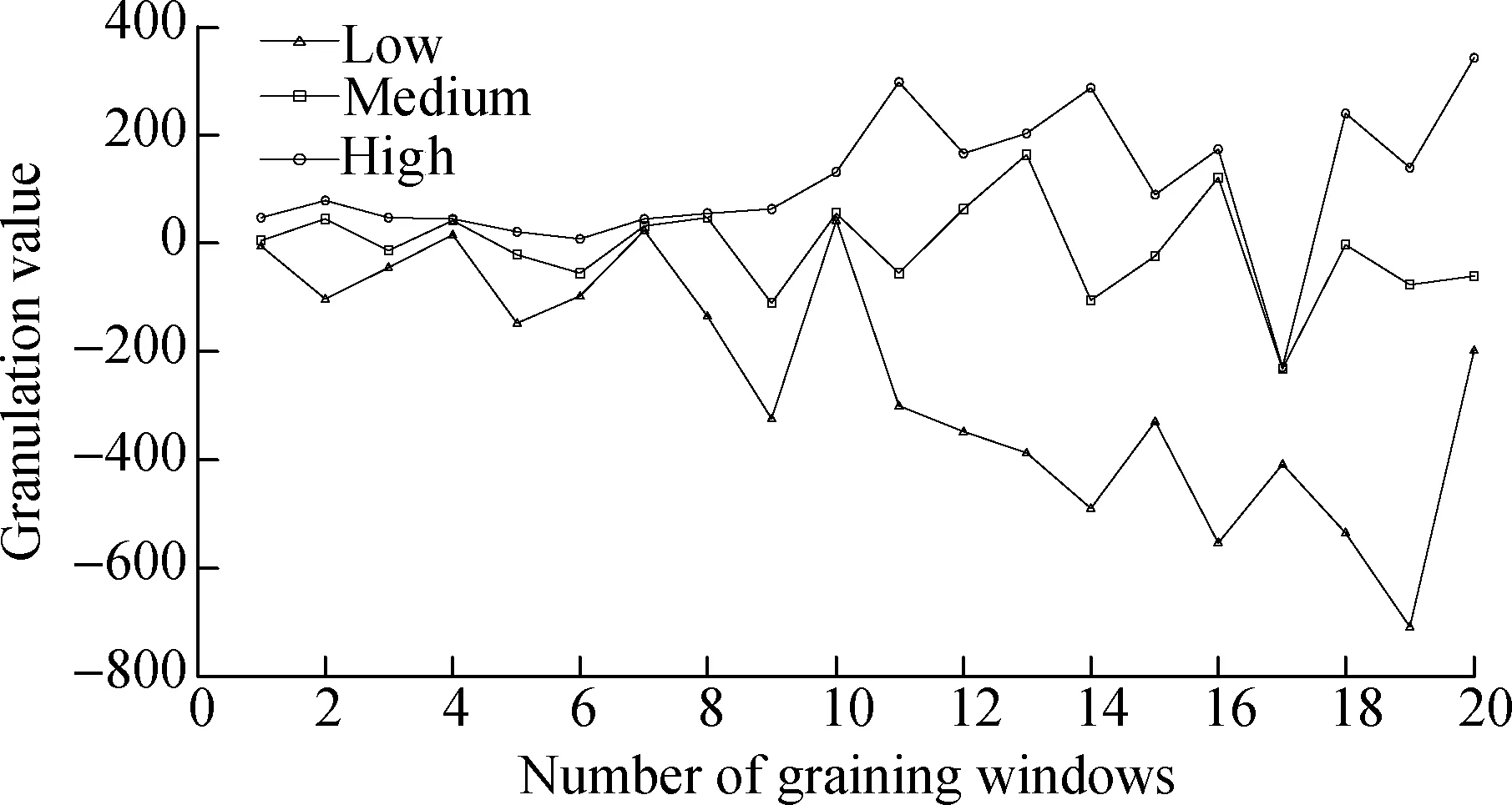
Fig.3 Granulation results

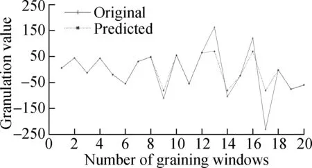
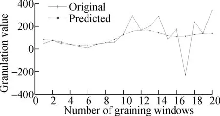
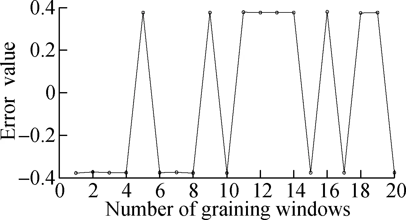
The SVR model is constructed by using fuzzy information particle data sets. Fuzzy information particles and window residuals are predicted so that the data can be normalized. Parameters are optimized by the Gale-Shapley algorithm. The output is shown in Fig.4.

It can be seen from Fig.4 that the overall residual prediction accuracy of the SVR model is high, where the low parameter prediction results are more accurate. However, when the windowed residual value changes greatly, the prediction values of the medium and high parameters will be inaccurate and the predicted values will be small, such as No.13,16,17 window. The SVR model uses the data from the previous window to complete the prediction of the data for the next window. This means that if the number of abnormal situations has a large fluctuation, the accuracy of the forecast will decrease.

The range of residual variation for the last three days is predicted. The low, medium, and high parameter predic-tions are -1.7, -5.9, and 127.2, respectively. Therefore, the SVR model is feasible for predicting the residual data, but there are also some shortcomings.

(a)

(b)

(c)

(d)

(e)

(f)Fig.4 Forecast results and errors of low, medium and high parameters.(a) Low parameter; (b) Medium parameter; (c) High parameter; (d) Low error; (e) Medium error;(f) High error

3.2.3 Combination model

The prediction value of the ARIMA model and the residual prediction value of the SVR are combined to predict the number of abnormal situations in the next three days (Time window is from the 61st to 63rd), as shown in Tab.6.

Tab.6 Prediction results of combined model

The experimental results show that the number of abnormal situations by the ARIMA model is 778, 761 and 805. It is similar to the actual numbers of abnormal situations (893, 758, 958), and the trends are consistent. The SVR model is used to correct the residual data. Through the combination of the two models, the overall prediction accuracy is increased by 4.6%. The prediction accuracy of the combined model is up to 94.4%.

4 Conclusion

This paper proposed a recognition model of survival situations, which focuses on the pre-recognition and the post-prediction. Experimental results show that the combined model effectively improves the accuracy of pre-recognition and post-prediction. The overall prediction accuracy is increased by 4.6%. The prediction accuracy of the combined model is up to 94.4%. However, there are still some flaws in our method. First, this paper mainly studies the internal environment of survivable system, but lacks the recognition of external attacks. Secondly, when the number of abnormal situations has a large fluctuation, the accuracy of the recognition will decline. Finally, the model is not suitable for predicting long-term survivability due to the uncertainty of situation data.